2. Types of Surveys Cross-sectional
surveys a specific population at a given point in time
will have one or more of the design components
stratification
clustering with multistage sampling
unequal probabilities of selection
Longitudinal
surveys a specific population repeatedly over a period of time
panel
rotating samples

3. Cross Sectional Surveys
Sampling Design Terminology

4. Methods of Sample Selection
Basic methods
simple random sampling
systematic sampling
unequal probability sampling
stratified random sampling
cluster sampling
two-stage sampling

5. Simple Random Sampling
Why?
basic building block of sampling
sample from a homogeneous group of units
How?
physically make draws at random of the units under study
computer selection methods: R, Stata

6. Systematic Sampling Why? easy
can be very efficient depending on the structure of the population
How?
get a random start in the population
sample every kth unit for some chosen number k

7. Additional Note Simplifying assumption:
in terms of estimation a systematic sample is often treated as a simple random sample
Key assumption:
the order of the units is unrelated to the measurements taken on them

8. Unequal Probability Sampling
Why?
may want to give greater or lesser weight to certain population units
two-stage sampling with probability proportional to size at the first stage and equal sample sizes at the second stage provides a self-weighting design (all units have the same chance of inclusion in the sample)
How?
with replacement
without replacement

9. With or Without Replacement?
in practice sampling is usually done without replacement
the formula for the variance based on without replacement sampling is difficult to use
the formula for with replacement sampling at the first stage is often used as an approximation
Assumption: the population size is large and the sample size is small – sampling fraction is less than 10%

10. Stratified Random Sampling
Why?
for administrative convenience
to improve efficiency
estimates may be required for each stratum
How?
independent simple random samples are chosen within each stratum

11. Example: Survey of Youth in Custody
first U.S. survey of youths confined to long-term, state-operated institutions
complemented existing Children in Custody censuses.
companion survey to the Surveys of State Prisons
the data contain information on criminal histories, family situations, drug and alcohol use, and peer group activities
survey carried out in 1989 using stratified systematic sampling

12. SYC Design strata sampling units
type (a) groups of smaller institutions
type (b) individual larger institutions
sampling units
strata type (a)
first stage – institution by probability proportional to size of the institution
second stage – individual youths in custody
strata type (b)
individual youths in custody
individuals chosen by systematic random sampling

13. Cluster Sampling Why? convenience and cost
the frame or list of population units may be defined only for the clusters and not the units
How?
take a simple random sample of clusters and measure all units in the cluster

14. Two-Stage Sampling Why? cost and convenience lack of a complete frame
How?
take either a simple random sample or an unequal probability sample of primary units and then within a primary take a simple random sample of secondary units

15. Synthesis to a Complex Design
Stratified two-stage cluster sampling
Strata
geographical areas
First stage units
smaller areas within the larger areas
Second stage units
households
Clusters
all individuals in the household

16. Why a Complex Design?
better cover of the entire region of interest (stratification)
efficient for interviewing: less travel, less costly
Problem: estimation and analysis are more complex

17. Ontario Health Survey carried out in 1990
health status of the population was measured
data were collected relating to the risk factors associated with major causes of morbidity and mortality in Ontario
survey of 61,239 persons was carried out in a stratified two-stage cluster sample by Statistics Canada

18. OHS Sample Selection
strata: public health units – divided into rural and urban strata
first stage: enumeration areas defined by the 1986 Census of Canada and selected by pps
second stage: dwellings selected by SRS
cluster: all persons in the dwelling

19. Longitudinal Surveys
Sampling Design

20. Schematic Representation

21. Schematic Representation

22. British Household Panel Survey
Objectives of the survey
to further understanding of social and economic change at the individual and household level in Britain
to identify, model and forecast such changes, their causes and consequences in relation to a range of socio-economic variables.

23. BHPS: Target Population and Frame
private households in Great Britain
Survey frame
small users Postcode Address File (PAF)

24. BHPS: Panel Sample
designed as an annual survey of each adult (16+) member of a nationally representative sample
5,000 households approximately
10,000 individual interviews approximately.
the same individuals are re-interviewed in successive waves
if individuals split off from original households, all adult members of their new households are also interviewed.
children are interviewed once they reach the age of 16
13 waves of the survey from 1991 to 2004

25. BHPS: Sampling Design
Uses implicit stratification embedded in two-stage sampling
postcode sector ordered by region
within a region postcode sector ordered by socio-economic group as determined from census data and then divided into four or five strata
Sample selection
systematic sampling of postcode sectors from ordered list
systematic sampling of delivery points (≈ addresses or households)

26. BHPS: Schema for Sampling

27. Survey Weights

28. Survey Weights: Definitions
initial weight
equal to the inverse of the inclusion probability of the unit
final weight
initial weight adjusted for nonresponse, poststratification and/or benchmarking
interpreted as the number of units in the population that the sample unit represents

29. Interpretation Interpretation
the survey weight for a particular sample unit is the number of units in the population that the unit represents

30. Effect of the Weights
Example: age distribution, Survey of Youth in Custody

31. Unweighted Histogram

32. Weighted Histogram

33. Weighted versus Unweighted

34. Observations the histograms are similar but significantly different
the design probably utilized approximate proportional allocation
the distribution of ages in the unweighted case tends to be shifted to the right when compared to the weighted case
older ages are over-represented in the dataset

35. Issues and Simple Examples from Graphical Methods
Survey Data Analysis
Issues and Simple Examples from Graphical Methods

36. Basic Problem in Survey Data Analysis

37. Issues iid (independent and identical distribution) assumption
the assumption does not not hold in complex surveys because of correlations induced by the sampling design or because of the population structure
blindly applying standard programs to the analysis can lead to incorrect results

38. Example: Rank Correlation Coefficient
Pay equity survey dispute: Canada Post and PSAC
two job evaluations on the same set of people (and same set of information) carried out in 1987 and 1993
rank correlation between the two sets of job values obtained through the evaluations was 0.539
assumption to obtain a valid estimate of correlation: pairs of observations are iid

39. Scatterplot of Evaluations
Rank correlation is 0.539

40. A Stratified Design with Distinct Differences Between Strata
the pay level increases with each pay category (four in number)
the job value also generally increases with each pay category
therefore the observations are not iid

41. Scatterplot by Pay Category

42. Correlations within Level
Correlations within each pay level
Level 2: –0.293
Level 3: –0.010
Level 4: 0.317
Level 5: 0.496
Only Level 4 is significantly different from 0

43. Graphical Displays first rule of data analysis common tools
always try to plot the data to get some initial insights into the analysis
common tools
histograms
bar graphs
scatterplots

44. Histograms unweighted weighted
height of the bar in the ith class is proportional to the number in the class
weighted
height of the bar in the ith class is proportional to the sum of the weights in the class

45. Body Mass Index measured by
weight in kilograms divided by square of height in meters
7.0 < BMI < 45.0
BMI < 20: health problems such as eating disorders
BMI > 27: health problems such as hypertension and coronary heart disease

46. BMI: Women

47. BMI: Men

48. BMI: Comparisons

49. Same principle as histograms
Bar Graphs
Same principle as histograms
unweighted
size of the ith bar is proportional to the number in the class
weighted
size of the ith bar is proportional to the sum of the weights in the class

50. Ontario Health Survey

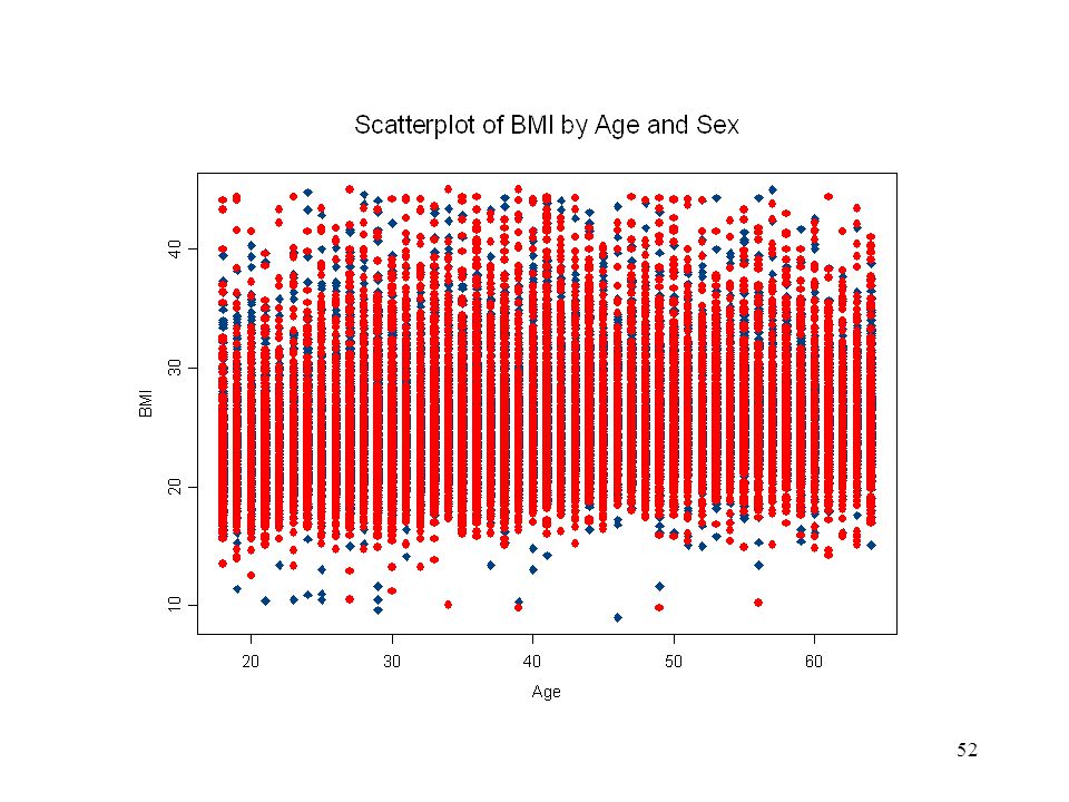
51. Scatterplots unweighted
plot the outcomes of one variable versus another
problem in complex surveys
there are often several thousand respondents

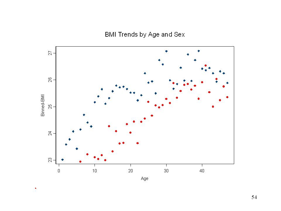
53. Solution bin the data on one variable and find a representative value
at a given bin value the representative value for the other variable is the weighted sum of the values in the bin divided by the sum of the weights in the bin

55. Bubble Plots
size of the circle is related to the sum of the surveys weights in the estimate
more data in the BMI range 17 to 29 approximately

56. Computing Packages
STATA and R

57. Available Software for Complex Survey Analysis
commercial Packages:
STATA
SAS
SPSS
Mplus
noncommercial Package R

58. STATA defining the sampling design: svyset example output:
svyset [pweight=indiv_wt], strata(newstrata) psu(ea) vce(linear)
output:
pweight: indiv_wt
VCE: linearized
Strata 1: newstrata
SU 1: ea
FPC 1: <zero>

59. R: survey package define the sampling design: svydesign output
wk1de<- svydesign(id=~ea,strata=~newstrata,weight=~indiv_wt,nest=T,data=work1)
output
> summary(wk1de)
Stratified 1 - level Cluster Sampling design
With (1860) clusters.
svydesign(id = ~ea, strata = ~newstrata, weight = ~indiv_wt,
nest = T, data = work1)

60. Syntax STATA: R: svy: estimate Example: least squares estimation
svyset [pweight=indiv_wt], strata(newstrata) psu(ea)
svy: regress dbmi bmi R:
svy***(*, design, data=, ...)
wk2de<-svydesign(id=~ea,strata=~newstrata,weight=~indiv_wt,nest=T,data=work2)
svyglm(dbmi~bmi, data=work2,design=wk2de)

61. Available Survey Commands
STATA
Descriptive
Yes
Regression
Yes (More)
Resampling
Longitudinal No
PMLE
Calibration

62. Contingency Tables and Issues of Estimation of Precision
Survey Data Analysis
Contingency Tables
and
Issues of Estimation of Precision

63. General Effect of Complex Surveys on Precision
stratification decreases variability (more precise than SRS)
clustering increases variability (less precise than SRS)
overall, the multistage design has the effect of increasing variability (less precise than SRS)

64. Illustration Using Contingency Tables
two categorical variables that can be set out in I rows and J columns
can get a survey estimate of the proportion of observations in the cell defined by the ith row and jth column:

65. Example: Ontario Health Survey
rows: five levels describing levels of happiness that people feel
columns: four levels describing the amount of stress people feel
Is there an association between stress and happiness?

66. STATA Commands

67. STATA Output table on stress and happiness
estimated proportions in the table with test statistic

68. Possible Test Statistics
adapt the classical test statistic
need the sampling distribution of the statistic
Wald Test
need an estimate of the variance-covariance matrix

69. Estimation of Variance or Precision
variance estimation with complex multistage cluster sample design:
exact formula for variance estimation is often too complex; use of an approximate approach required
NOTE: taking account of the design in variance estimation is as crucial as using the sampling weights for the estimation of a statistic

70. Some Approximate Methods
Taylor series methods
Replication methods
Balanced Repeated Replication (BRR)
Jackknife
Bootstrap

71. Replication Methods
you can estimate the variance of an estimated parameter by taking a large number of different subsamples from your original sample
each subsample, called a replicate, is used to estimate the parameter
the variability among the resulting estimates is used to estimate the variance of the full-sample estimate
covariance between two different parameter estimates is obtained from the covariance in replicates
the replication methods differ in the way the replicates are built

72. Assumptions
The resulting distribution of the test statistic is based on having a large sample size with the following properties
the total number of first stage sampled clusters (or primary sampling units) is assumed large
the primary sample size in each stratum is small but the number of strata is large
the number of primary units in a stratum is large
no survey weight is disproportionately large

73. Possible Violations of Assumptions
the complex survey (stratified two-sample sampling, for example) was done on a relatively small scale
a large-scale survey was done but inferences are desired for small subpopulations
stratification in which a few strata (or just one) have very small sampling fractions compared to the rest of the strata
The sampling design was poor resulting in large variability in the sampling weights

74. Linear and Logistic Regression
Survey Data Analysis
Linear and Logistic
Regression

75. General Approach
form a census statistic (model estimate or expression or estimating equation)
for the census statistic obtain a survey estimate of the statistic
the analysis is based on the survey estimate

76. Regression Use of ordinary least squares can lead to
badly biased estimates of the regression coefficients if the design is not ignorable
underestimation of the standard errors of the regression coefficient if clustering (and to a lesser extent the weighting) is ignored

77. Example: Ontario Health Survey
Regress desired body mass index (DBMI) on body mass index (BMI)

78. Simple Linear Regression Model
typical regression model
linear relationship plus random error
errors are independent and identically distributed

79. Census Statistic census estimate of the slope parameter 
Problem: the assumption of independent errors in the population does not hold
Solution: the least squares estimate is a consistent estimate of the slope 

80. Survey Estimate the census estimate B is now the parameter of interest
the survey estimate is given by
estimate obtained from an estimating equation
the estimate of variance cannot be taken from the analysis of variance table in the regression of y on x using either a weighted or unweighted analysis

81. Variance Estimation
Again, estimate of the variance of b is obtained from one of the following procedures
Taylor linearization
Jackknife
BRR
Bootstrap

82. Issues in Analysis
application of the large sample distributional results
small survey
regression analysis on small domains of interest
multicollinearity
survey data files often have many variables recorded that are related to one another

83. Multicollinearity Example: Ontario Health Survey
Two regression models: regress desired body mass index on
actual body mass index, age, gender, marital status, smoking habits, drinking habits, and amount of physical activity
all of the above variables plus interaction terms: marital status by smoking habits, marital status by drinking habits, physical activity by age

84. Partial STATA Output
No interaction terms
Interaction terms present

85. Comparison of Domain Means
Domains and Strata
both are nonoverlapping parts or segments of a population
usually a frame exists for the strata so that sampling can be done within each stratum to reduce variation
for domains the sample units cannot be separated in advance of sampling
Inferences are required for domains.

86. Regression Approach
use the regression commands in STATA and declare the variables of interest to be categorical
example: DBMI relative to BMI related to sex and happiness index
STATA commands

87. STATA Output

88. Logistic Regression probability of success pi for the ith individual
vector of covariates xi associated with ith individual
dependent variable must be 0 or 1, independent variables xi can be categorical or continuous
Does the probability of success pi depend on the covariates xi – and in what way?

89. Census Parameter Obtained from the logistic link function
and the census likelihood equation for the regression parameters
Note: it is the log odds that is being modeled in terms of the covariate

90. Example: Ontario Health Survey
How does the chance of suffering from hypertension depend on:
body mass index
age
gender
smoking habits
stress
a well-being score that is determined from self-perceived factors such as the energy one has, control over emotions, state of morale, interest in life and so on

91. STATA Commands

92. STATA Output part I

93. STAT Output part II

94. GEE: Generalized Estimating Equations
Dependent or response variable
well-being measured on a 0 to 10 scale
focus is on women only
Independent or explanatory variables’
has responsibility for a child under age 12 (yes = 1, no = 2)
marital status (married = 1, separated = 2, divorced = 3, never married = 5 [widowed removed from the dataset])
employment status (employed = 1, unemployed = 2, family care = 3)
STATA syntax
tsset pid year, yearly
xi: xtgee wellbe i.mlstat i.job i.child i.sex [pweight = axrwght], family(poisson) link(identity) corr(exchangeable)

95. GEE Results

96. For each type of initial marital status
Married
Separated or divorced
Never married

97. Cox Proportional Hazards Model
Dependent or outcome variable
time to breakdown of first marriage
Independent or explanatory variables
gender
race (white/non-white)
Age in 1991 (restricted to 18 – 60)
financial position: comfortable=1, doing alright=2, just about getting by=3, quite difficult=4, very difficult =5

98. STATA Commands Command for survival data set up
Command for Cox proportional hazards mode

99. STATA Output