1. Compiling Graphical Models Adnan Darwiche University of California, Los Angeles UAI06 Tutorial

2. Compilation: Historical Motivation Separate inference into two phases: Offline: Compile model into a structure Online: Use structure to answer queries Goal: Push as much work into offline phase to optimize online inference time Best initial example: Offline: Compile a Bayesian network into a jointree Online: Use jointree to answer multiple queries efficiently

3. Compilation: Modern Motivation Exploit model structure in inference: Global structure: Exhibited in model topology Measured by treewidth Exploited by most (non-compilation) algorithms Local structure: Exhibited in model parameters Type 1: Determinism Type 2: Context-specific independence Local structure is best exploited in the context of compilation: main theme

4. Compilation: Theoretical Implications Unifies inference paradigms Variable elimination Jointree (Tree clustering) Conditioning Compilation as a trace of classical inference

5. Bayesian Networks Battery Age Alternator Fan Belt Battery Charge Delivered Battery Power Starter Radio LightsEngine Turn Over Gas Gauge Gas Fuel Pump Fuel Line Distributor Spark Plugs Engine Start Local Knowledge

6. Bayesian Networks Battery Age Alternator Fan Belt Battery Charge Delivered Battery Power Starter Radio LightsEngine Turn Over Gas Gauge Gas Fuel Pump Fuel Line Distributor Spark Plugs Engine Start ON OFF OK WEAK DEAD Lights Battery Power.99.01.20.80 01 If Battery Power = OK, then Lights = ON (99%) ….

7. Bayesian Networks Battery Age Alternator Fan Belt Battery Charge Delivered Battery Power Starter Radio LightsEngine Turn Over Gas Gauge Gas Fuel Pump Fuel Line Distributor Spark Plugs Engine Start

8. Global Structure: Treewidth w

9. Battery Age Alternator Fan Belt Battery Charge Delivered Battery Power Starter Radio LightsEngine Turn Over Gas Gauge Gas Fuel Pump Fuel Line Distributor Spark Plugs Engine Start Local Structure: CSI and Determinism

10. Battery Age Alternator Fan Belt Battery Charge Delivered Battery Power Starter Radio LightsEngine Turn Over Gas Gauge Gas Fuel Pump Fuel Line Distributor Spark Plugs Engine Start Context Specific Independence (CSI) Local Structure: CSI and Determinism

11. Battery Age Alternator Fan Belt Battery Charge Delivered Battery Power Starter Radio LightsEngine Turn Over Gas Gauge Gas Fuel Pump Fuel Line Distributor Spark Plugs Engine Start ON OFF OK WEAK DEAD Lights Battery Power.99.01.20.80 01 If Battery Power = Dead, then Lights = OFF Determinism

12. Todays Models … Characterized by: Richness in local structure (determinism, CSI) Massiveness in size (100,000s variables not uncommon) High connectivity (treewidth > 50, > 100) Enabled by: High level modeling tools: relational, first order New application areas (synthesis): Bioinformatics (e.g. linkage analysis) Sensor networks Exploiting local structure a must!

13. High Order Specifications: Relational Models… burglary(v)=0.005; alarm(v)=(burglary(v):0.95,0.01); calls(v,w)= (neighbor(v,w): (prankster(v)): (alarm(w):0.9,0.05), (alarm(w):0.9,0)),0); alarmed(v)= n-or{calls(w,v)|w:neighbor(w,v)} burglary(v)=0.005; alarm(v)=(burglary(v):0.95,0.01); calls(v,w)= (neighbor(v,w): (prankster(v)): (alarm(w):0.9,0.05), (alarm(w):0.9,0)),0); alarmed(v)= n-or{calls(w,v)|w:neighbor(w,v)} Primula

15. Friends and Smokers ( Richardson & Domingos, 2004) M individuals Relations such as smokes(p), cancer(p), friend(p 1,p 2 ) Logical constraints such as: if one of p's friends smokes, then p smokes. Sample Query: probability that given person has cancer

16. Students (Pasula & Russell, 2001) P professors S students Various relations, such as famous(p), well- funded(p), success(s), advises(p,s) Sample Query: probability a professor is well-funded given success of advised students 12.9663 3.2120 1.8439 0.2885 0.0930 0.0530 Online Time (sec) 3336,450,23164,32517,69323362,30206-24 1416,936,50433,3539,20917633,45406-12 75,236,25738,88910,73414838,16805-20 32,531,23020,2795,62412820,68805-10 3815,46121,1155,85910121,07004-16 2445,41011,0993,0997211,56604-08 Offline Time (min) AC Edges Cnf Clauses CNF Vars Treewidth w Network params Students- Profs

17. Ordering genes on a chromosome and determining distance between them Useful for predicting and detecting diseases Associating functionality of genes with their location on the chromosome Gene 1 Gene 2 Gene 3 Genetic Linkage Analysis

18. Pedigrees + Phenotype + Genotype

20. DBNs from Speech Applications

21. Coding Networks

22. Tutorial Outline Theoretical foundations Online query answering algorithms Offline compilation algorithms Applications Concluding remarks

23. Theoretical Foundations Graphical Model (Bayesian, Markov Networks): Is a Multi-Linear Function (MLF) Compiled Model: Is an Arithmetic Circuit (AC) Compilation process: Factoring MLF into AC

24. Multi-Linear Functions Arithmetic Circuits AB * * ** + ++ * ** * Factoring A Differential Approach to Inference in Bayesian Networks JACM-03 (Darwiche)

25. Factoring Multi-linear Functions (MLFs) a + ad + abd + abcd MLF: * + * abdc1 + Arithmetic Circuit (AC) An MLF has an exponential number of terms, yet it may be represented by an AC with polynomial size! A graphical model defines an MLF Evaluating the MLF for a given evidence gives the probability of evidence The inference problem can be formulated as factoring the MLF of a graphical model Circuit Complexity: Size of smallest AC that computes the MLF

26. Pr(a) =.03 +.27 =.3 false B.03.27 A.56.14 true false Pr(.) false true Graphical Models as MLFs

27. Pr(~b) =.27 +.14 =.41 false B.03.27 A.56.14 true false true Pr(.) Graphical Models as MLFs

28. .03λ a λ b +.27λ a λ ~b +.56λ ~a λ b +.14λ ~a λ ~b false B.03 A true false true.27.14.56 λ a* λ b *.03 λ a* λ ~ b *.27 λ ~ a* λ b *.56 λ ~ a* λ ~ b*.14 F (λ ~a, λ ~b, λ a, λ b ) = Pr(.) Graphical Models as MLFs

29. =.03λ a λ b +.27λ a λ ~b +.56λ ~a λ b +.14λ ~a λ ~b F (λ ~a, λ ~b, λ a, λ b ) Pr(a,~b) = F (λ ~a :0, λ ~b :1, λ a :1, λ b :0) =.27 Pr(a) = F (λ ~a :0, λ ~b :1, λ a :1, λ b :1) =.03+.27

30. A B C θ b|a θaθa θ c|a ABCPr(.) abcθ a θ b|a θ c|a ab~cθ a θ b|a θ ~c|a a~bcθ a θ ~b|a θ c|a a~b~cθ a θ ~b|a θ ~c|a...…

31. A B C θ b|a θaθa θ c|a ABCPr(.) abc λ a λ b λ c θ a θ b|a θ c|a ab~c λ a λ b λ ~c θ a θ b|a θ ~c|a a~bc λ a λ ~b λ c θ a θ ~b|a θ c|a a~b~c λ a λ ~b λ ~c θ a θ ~b|a θ ~c|a...…

32. F = λ a λ b λ c θ a θ b|a θ c|a + λ a λ b λ ~c θ a θ b|a θ ~c|a + λ a λ ~b λ c θ a θ ~b|a θ c|a + λ a λ ~b λ ~c θ a θ ~b|a θ ~c|a …. A B C

33. F = λ a λ b λ c λ d θ a θ b|a θ c|a θ d|bc + λ a λ b λ c λ ~d θ a θ b|a θ c|a θ ~d|bc + …. A B C D Each term has 2n variables (n indicators, n parameters) Each variable has degree one (multi-linear function) θaθa θ b|a θ c|a θ d|bc

34. Multi-Linear Functions Arithmetic Circuits AB * * ** + ++ * ** * Factoring

35. Online Query Answering Complexity: Time and space linear in the AC size Queries: Probability of evidence, with evidence flipping/fast retraction Variable and family marginals MPE: most probable explanation Sensitivity analysis (derivatives)

36. Evaluating the Polynomial

37. PR: Probability of Evidence Battery Age Alternator Fan Belt Battery Charge Delivered Battery Power Starter Radio LightsEngine Turn Over Gas Gauge Gas Fuel Pump Fuel Line Distributor Spark Plugs Engine Start Pr(e)

38. The Partial Derivatives

39. PR: Probability of Evidence Flips Battery Age Alternator Fan Belt Battery Charge Delivered Battery Power Starter Radio LightsEngine Turn Over Gas Gauge Gas Fuel Pump Fuel Line Distributor Spark Plugs Engine Start Pr(e) X

40. PR: Probability of Evidence Flips Battery Age Alternator Fan Belt Battery Charge Delivered Battery Power Starter Radio LightsEngine Turn Over Gas Gauge Gas Fuel Pump Fuel Line Distributor Spark Plugs Engine Start Pr(e-X,x) X

41. The Partial Derivatives

42. PR: Family Marginals Battery Age Alternator Fan Belt Battery Charge Delivered Battery Power Starter Radio LightsEngine Turn Over Gas Gauge Gas Fuel Pump Fuel Line Distributor Spark Plugs Engine Start U X Pr(e,x,u)

43. Multi-Linear Functions Arithmetic Circuits AB * * ** + ++ * ** * Factoring

44. * * * * + + + * * * * Circuit Evaluation and Differentiation: Marginals.3 1.1 1.9.8 1.2 0.7.3.3.1.9.8.2 0 1 1.3 0 1 1 1 1.3.3 0 0 1 1.3.03.30.270.70 Two passes only: probability of evidence (with evidence flipping) Node marginals Family marginals Sensitivity

45. Efficient Eval/Diff Schemes Assume alternating levels of +/* nodes, with one parent per *node Method A: Two registers per +node (no registers for *nodes) Method B: One register per node (use for values in upward pass, then override with derivatives in downward pass) Method C: One register per node, one bit per *node

46. .3 1.1 1.9.8 1.2 0.7 ** ** m mm ** * *.27.3.1.9.8.2 0.9.8.27 0 Circuit Optimization: MPE * **

47. m * m **

48. Custom Hardware for Evaluating ACs Adharapurapu, Ercegovac (2004)

49. Offline Compilation Factoring MLFs into ACs: Jointree: Embeds AC Variable Elimination: Trace is an AC Recursive Conditioning: Trace is an AC Reduction to Logic: CNF to d-DNNF compilation

50. Compiling using Jointrees Classical Jointree Algorithm: Convert model into jointree Jointree propagation (two-passes) Modern interpretation: Jointree embeds an AC that factors MLF Jointree propagation is evaluating/differentiating embedded AC

51. AB A AB root A Jointree Embeds an AC… ACAD AE AB A AB Inward-pass evaluates circuit Outward-pass differentiates circuit [Hugin, Shenoy Shafer,…] A Differential Semantics to Jointree Algorithms AIJ-04 (with James Park)

52. Efficient Eval/Diff Schemes Assume alternating levels of +/* nodes, with one parent per *node Method A: Two registers per +node (no registers for *nodes) Method B: One register per node (use for values in upward pass, then override with derivatives in downward pass) Method C: One register per node, one bit per *node

53. Jointree Flavors Shenoy-Shafer: Method A Hugin: Method B (looses information) Zero-Conscious Hugin (new): Method C (best of A,B)

54. Compiling using Variable Elimination (VE) VE operates on factors: Mappings from variable instantiations to real numbers VE performs two operations on factors: Multiply two factors Sum-Out a variable from factor Factors have different representations: Tables More structured representations (decision trees/graphs) Overhead problem for structured factors

55. A B true false A.3.7 TATA Tabular Factors false B.1.9 A.8.2 true false TBTB true

56. X Z.1.9 Y.5 Z Structured Factors: Algebraic Decision Diagrams (ADDs)

57. NetworkMax ClustVarsCardTotal Parms%Det%Distinct alarm7.2372...47520.924.6 bm2010052...2697299.6100 diabetes17.24133...2146106978.217.6 hailfinder11.7562...11374115.726.9 mildew21.4353...10054715893.225.1 mm2312202...2832698.775 munin126.81891...211946666.561.2 munin218.610032...218392063.369.5 munin317.810441...218585563.171.3 munin421.410411...219818364.565.3 pathfinder151092...639785156.15.1 pigs17.44413...3842756.223.9 students223762...2261690.779.3 tcc4f101052...232360.435.6 water19.9323...4134845457 Networks with Local Structure

58. VE: Tabular vs ADD Representations of Factors TabularADD NetworkTime (ms) Improvement alarm313600.086 barley30714,0490.022 bm-5-34,8926587.435 diabetes94933,2200.029 hailfinder485150.093 link1,6882,6580.635 mm-3-8-32,1668432.569 mildew7292,6020.001 munin11551,2550.124 munin22043,1700.064 munin33505,0490.069 munin44064,3610.093 pathfinder515,2130.01 pigs695970.116 st-3-21863620.514 tcc4f291530.19 water761,0150.075

59. Compiling using Variable Elimination (VE) By using symbolic factors and corresponding operations: VE compiles out an AC VE with tabular factors: Generates ACs similar to those embedded in jointree VE with structured factors: Generates much smaller ACs Overhead pushed into offline phase

60. A B true false A.3.7 TATA Factors false B.1.9 A.8.2 true false TBTB true

61. A B false ATATA θ a * λ a θ ~a * λ ~a false BA true false TBTB true θ ~b|a * λ ~b θ b|~a * λ b θ b|a * λ b θ ~b|~a * λ ~b Symbolic Factors

62. true false ATBTB θ b|a * λ b + θ ~b|a * λ ~b θ b|~a * λ b + θ ~b|~a * λ ~b false BA true false TBTB true θ ~b|a * λ ~b θ b|~a * λ b θ b|a * λ b θ ~b|~a * λ ~b Summing out B Summing out Variable B

63. *= Multiplying Factors true false AT A T B θ a * λ a *( θ b|a * λ b + θ ~b|a * λ ~b ) θ ~ a * λ ~ a *( θ b|~a * λ b + θ ~b|~a * λ ~b ) true false ATBTB θ b|a * λ b + θ ~b|a * λ ~b θ b|~a * λ b + θ ~b|~a * λ ~b true false A TATA θ a *λ a θ ~a *λ ~a

64. θ a * λ a * ( θ b|a * λ b + θ ~b|a * λ ~b ) + θ ~ a * λ ~ a ( θ b|~a * λ b + θ ~b|~a * λ ~b ) true false AT A T B θ a * λ a * ( θ b|a * λ b + θ ~b|a * λ ~b ) θ ~ a * λ ~ a * ( θ b|~a * λ b + θ ~b|~a * λ ~b ) Summing out Variable A

65. VE factors MLF into AC (Bottom up Construction) AB * * ** + ++ * ** * Factoring Time and space complexity of generating AC is similar to Variable Elimination: Exponential only in treewidth Generated ACs similar to those embedded in Jointree Recall: AC can be used to answer multiple queries!

66. X Z.1.9 Y.5 Z Structured Factors: Algebraic Decision Diagrams (ADDs)

67. X ZY Z Symbolic ADD Modify standard ADD operations (multiply, sum-out) to operate on symbolic ADDs Run variable elimination with symbolic ADDs Compile out an AC Asymptotic complexity is no worse than variable elimination Overhead of ADDs is pushed into offline phase Generated AC can be much smaller Online inference can be much faster

68. NetworkMax ClustVarsCardTotal Parms%Det%Distinct alarm7.2372...47520.924.6 bm2010052...2697299.6100 diabetes17.24133...2146106978.217.6 hailfinder11.7562...11374115.726.9 mildew21.4353...10054715893.225.1 mm2312202...2832698.775 munin126.81891...211946666.561.2 munin218.610032...218392063.369.5 munin317.810441...218585563.171.3 munin421.410411...219818364.565.3 pathfinder151092...639785156.15.1 pigs17.44413...3842756.223.9 students223762...2261690.779.3 tcc4f101052...232360.435.6 water19.9323...4134845457 Networks with Local Structure

69. TabularADD NetworkTime (ms) Improvement alarm313600.086 barley30714,0490.022 bm-5-34,8926587.435 diabetes94933,2200.029 hailfinder485150.093 link1,6882,6580.635 mm-3-8-32,1668432.569 mildew7292,6020.001 munin11551,2550.124 munin22043,1700.064 munin33505,0490.069 munin44064,3610.093 pathfinder515,2130.01 pigs695970.116 st-3-21863620.514 tcc4f291530.19 water761,0150.075 Tabular vs ADD: Standard VE

70. Time (s)AC size NetworkAceADD-VEImprov.Tabular-VEADD-VEImprov. alarm0.33.90.13,5343,0301.2 barley8,190.20122.866.766,467,77724,653,7442.7 bm-5-30.860.175,591,75014,8365095.2 diabetes1,710.00110.315.534,728,95717,219,0422 hailfinder0.71.20.572,75525,9922.8 link-699.7-127,262,77789,097,4501.4 mildew3,125.20218.914.316,094,5923,352,3304.8 mm-3-8-31.511.90.136,635,566108,428337.9 munin11,005.10316.73.2 1,260,407,123 31,409,97040.1 munin2198.431.76.320,295,4265,662,2183.6 munin3188.417.610.716,987,0883,503,2424.8 munin420537.85.476,028,5326,869,76011.1 pathfinder4.95.80.9796,58844,46817.9 pigs23.1102.34,925,3882,558,6801.9 st-3-20.52.40.219,374,93422,070877.9 tcc4f0.91.10.833,40822,6121.5 water320.70.115,996,054170,42893.9 Tabular vs ADD: VE Compilations

71. NetworkJointreeADD-VEImprov. alarm166325.2 barley65,22635,2091.9 bm-5-389,593831079.4 diabetes29,31620,4211.4 hailfinder245703.5 link223,542175,7691.3 mildew10,0774,5222.2 mm-3-8-334,001198171.7 munin1669,91537,45117.9 munin217,8577,1802.5 munin313,3514,9452.7 munin442,7548,6834.9 pathfinder1,33210213.1 pigs3,0202,8141.1 st-3-217,53682213.9 tcc4f281733.8 water16,67625166.4 ADD-VE vs Jointree: Online Inference Time (ms) Computing all marginals, for 16 pieces of random evidence Work on structured representations of factors is now much more relevant and practical.

72. Compiling by Reduction to Logic Algebraic: MLFs / ACs Logical: CNF / d-DNNF Factoring MLF into AC can be reduced to factoring CNF into d-DNNF CNF to d-DNNF compilers are very powerful (natural for exploiting determinism and CSI)

73. Compiler: http://reasoning.cs.ucla.edu/c2d d-DNNF CNF Multi-Linear Function Arithmetic Circuit Encode Decode Reduction to Logic

74. a c + a b c + c Multi-linear function:Propositional theory: c ^ (a b) Encode c b 1 a 1 Arithmetic Circuit Decode c b b a a Smooth d-DNNF Compile MLFs ACs CNFs d-DNNF

75. or and A A or and B C or and D E or BD and, Deterministic, Decomposable NNF

76. or and A A or and B C or and D E or BD and, Deterministic, Decomposable NNF Deterministic: Disjuncts are logically disjoint

77. or and A A or and B C or and D E or BD and Deterministic, Decomposable NNF B C B D E D Decomposable: Conjuncts share no variables Compiling CNFs into d-DNNFs AAAI-02, ECAI-04 Compiler at http://reasoning.cs.ucla.edu/c2dhttp://reasoning.cs.ucla.edu/c2d

78. A B C A D E Recursive Conditioning for Compilation or B C D E B C A and A B C D E B C D E

79. and 0 A B 1 DB C D E And-Or Graphs

80. Propositional Encoding of Multi-Linear Functions Propositional theory: Δ = c ^ (a b) Encodes: F = a c + a b c + c abcEncodes TTT abc TTFab TFT ac TFFa FTTbc FTFb FFT c FFF1

81. A B F = λ a λ b θ a θ b|a + λ a λ ~b θ a θ ~b|a + λ ~a λ b θ ~a θ b|~a + λ ~a λ ~b θ ~a θ ~b|~a λ a λ ~a ¬ λ a ¬ λ ~a λ b λ ~b ¬ λ b ¬ λ ~b λ a θ a λ ~a θ ~a λ a ^ λ b θ b|a λ a ^ λ ~ b θ ~ b|a λ ~ a ^ λ b θ b|~a λ ~ a ^ λ ~ b θ ~ b|~a Encoding Model as CNF

82. Why Logic? Encoding local structure is easy: Determinism encoded by adding clauses: CSI encoded by collapsing variables: A natural environment to exploit local structure: DD-backtracking, clause learning, … Non-structural decomposition Non-structural (formula) caching

83. ABC S 0.95 c abc A Pr(S|A,B,C) BC a a a a a a a b b b b b b b c c c c c c 0.95 0.20 0.05 0.00 Tabular CPT -Functional constraints -Context-specific independence s|abe Local Structure

84. 0.95 c abc A Pr(S|A,B,E) BC a a a a a a a b b b b b b b c c c c c c 0.95 0.20 0.05 0.00 Tabular CPT λ ~a λ b λ c λ s θ s|~abc ¬ λ ~a ¬ λ b ¬ λ c ¬ λ s Determinism

85. 0.95 c abc A Pr(S|A,B,C) BC a a a a a a a b b b b b b b c c c c c c 0.95 0.20 0.05 0.00 Tabular CPT λ a λ b λ s θ s|ab λ a λ b λ c λ s θ s|abc λ a λ b λ ~c λ s θ s|ab~c Context-Specific Independence

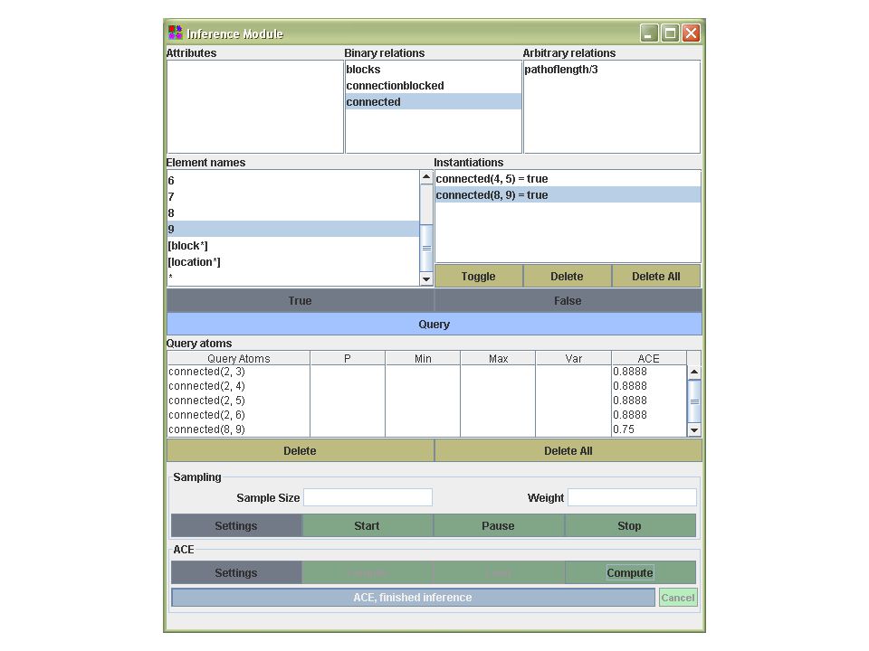
86. X Y Belief network x x x y x|y …. CNF Smooth d-DNNF x y x|y x x y x|y Arithmetic Circuit The Ace System: http://reasoning.cs.ucla.edu/ace

87. Time (s)AC size NetworkAceADD-VEImprov.Tabular-VEADD-VEImprov. alarm0.33.90.13,5343,0301.2 barley8,190.20122.866.766,467,77724,653,7442.7 bm-5-30.860.175,591,75014,8365095.2 diabetes1,710.00110.315.534,728,95717,219,0422 hailfinder0.71.20.572,75525,9922.8 link-699.7-127,262,77789,097,4501.4 mildew3,125.20218.914.316,094,5923,352,3304.8 mm-3-8-31.511.90.136,635,566108,428337.9 munin11,005.10316.73.2 1,260,407,123 31,409,97040.1 munin2198.431.76.320,295,4265,662,2183.6 munin3188.417.610.716,987,0883,503,2424.8 munin420537.85.476,028,5326,869,76011.1 pathfinder4.95.80.9796,58844,46817.9 pigs23.1102.34,925,3882,558,6801.9 st-3-20.52.40.219,374,93422,070877.9 tcc4f0.91.10.833,40822,6121.5 water320.70.115,996,054170,42893.9 ADD-VE vs Logic (Ace): Compile Times

88. NetworkNodesParametersMax Cluster mastermind_04_08_031418980226 mastermind_06_08_0318141275437 mastermind_10_08_0326061865854 mastermind_03_08_0422881600831 mastermind_04_08_0426161848839 mastermind_03_08_0536922618640 students_03_02376261625 students_03_121346985659 students_04_16282721070101 students_05_20506438168148 students_06_24820162302233 blockmap_05_031005697223 blockmap_10_0368484875852 blockmap_15_031878713243668 blockmap_20_034335630722092 blockmap_22_0359404423452104 ADD-VE vs Logic (Ace)

89. Network Offline Time (min) AC NodesAC Edges Online Inference Time (s) mastermind_04_08_03171,666541,3560.05 mastermind_06_08_031258,2281,523,8880.15 mastermind_10_08_0331,293,3234,315,5660.68 mastermind_03_08_042186,3514,859,2010.3 mastermind_04_08_045932,35519,457,3081.73 mastermind_03_08_05101,359,39155,417,6394.33 students_03_0217,92737,2810.01 students_03_12124,219113,8760.02 students_04_163181,166815,4610.09 students_05_2071,319,8345,236,2571.84 students_06_24339,922,23336,450,23112.97 blockmap_05_0312,83320,6360.01 blockmap_10_03217,749974,8170.06 blockmap_15_03647,4757,643,3070.38 blockmap_20_0330105,60240,172,4342.45 blockmap_22_0361144,13676,649,3024.67 ADD-VE vs Logic (Ace)

90. Effect of Local Structure Local Structure Encoded PathfinderWaterMunin4 None981,17813,777,166116,136,985 Det + CSI42,810 (4%) 134,140 (1%) 5,762,690 (5%) Det130,380 (13%) 138,501 (1%) 9,997,267 (9%) CSI200,787 (20%) 11,111,104 (81%) 17,612,036 (15%)

91. Compilation vs Direct Inference Grid problems here…

92. Compilation vs Direct Inference Grid size Treewidth w DetCachet (sec) Ace offline (sec) Ace online (sec) Offline/ Online 16x162550%22362202.0721079 22x223675%27573492.1782024 34x346090%1584790.4193783 Average over 10 random instances for each grid Ace available at http://reasoning.cs.ucla.edu/acehttp://reasoning.cs.ucla.edu/ace

93. Applications Relational Models Diagnosis Genetic Linkage Analysis

94. burglary(v)=0.005; alarm(v)=(burglary(v):0.95,0.01); calls(v,w)= (neighbor(v,w): (prankster(v)): (alarm(w):0.9,0.05), (alarm(w):0.9,0)),0); alarmed(v)= n-or{calls(w,v)|w:neighbor(w,v)} burglary(v)=0.005; alarm(v)=(burglary(v):0.95,0.01); calls(v,w)= (neighbor(v,w): (prankster(v)): (alarm(w):0.9,0.05), (alarm(w):0.9,0)),0); alarmed(v)= n-or{calls(w,v)|w:neighbor(w,v)} Primula/Ace: Upcoming Release

99. Friends and Smokers ( Richardson & Domingos, 2004) M individuals Relations such as smokes(p), cancer(p), friend(p 1,p 2 ) Logical constraints such as: if one of p's friends smokes, then p smokes. Sample Query: probability that given person has cancer

100. Friends & Smokers MNetwork params Treewidth w CNF Vars Cnf Clauses AC Edges Online Time (sec) Offline Time (sec) 134312311800.03 41,552134141,3902930.0030.44 77,714361,9956,9161,2950.0061.92 1021,760705,56519,5253,5120.0056.66 1346,93011811,93442,1337,4300.01312.8 1686,46417221,91277,65613,5350.02221.68 19143,60224436,309129,01022,3130.03538.36 22221,58431655,935199,11134,2500.05890.67 25323,65041281,600290,87549,8320.079162.45 28453,040528114,114407,21869,5450.114274.2 29502,802560126,614451,96577,1180.119275.17

101. Students (Pasula & Russell, 2001) P professors S students Various relataios, such as famous(p), well- funded(p), success(s), advises(p,s) Sample Query: probability a professor is well-funded given success of advised students

102. Students Students- Profs Network params Treewidth w CNF Vars Cnf Clauses AC Edges Online Time (sec) Offline Time (min) 04-0811,566723,09911,099445,4100.05302 04-1621,0701015,85921,115815,4610.09303 05-1020,6881285,62420,2792,531,2300.28853 05-2038,16814810,73438,8895,236,2571.84397 06-1233,4541769,20933,35316,936,5043.212014 06-2462,30223317,69364,32536,450,23112.966333

103. Diagnosis QMR-like: Effect of Encoding Evidence 600 diseases (D) and 4100 features (F) Feature F j is a noisy-or of parent diseases D i (11 parents chosen randomly) Sample Query: probability of disease given partial evidence on features. D1D1 D2D2 D3D3 DmDm … F1F1 F2F2 FnFn …

104. Treewidth: 586-589 CNF variables: 94,900 CNF clauses: 188,600 No. True Features AC Edges Online Time (sec) Offline Time (sec) 048,1000.0523.73 352,8300.0523.86 657,6380.0523.81 962,5470.0523.82 1267,6320.0524.19 1573,3210.0423.6 1881,6290.0524.95 21109,3350.0530.95 25434,4450.08155.12 271,141,6740.17469.7 281,691,8330.23728.52 292,352,8200.31,046.93 Diagnosis QMR-like: Effect of Encoding Evidence

105. Ordering genes on a chromosome and determining distance between them Useful for predicting and detecting diseases Associating functionality of genes with their location on the chromosome Gene 1 Gene 2 Gene 3 Genetic Linkage Analysis

106. Pedigrees + Phenotypes + Genotypes

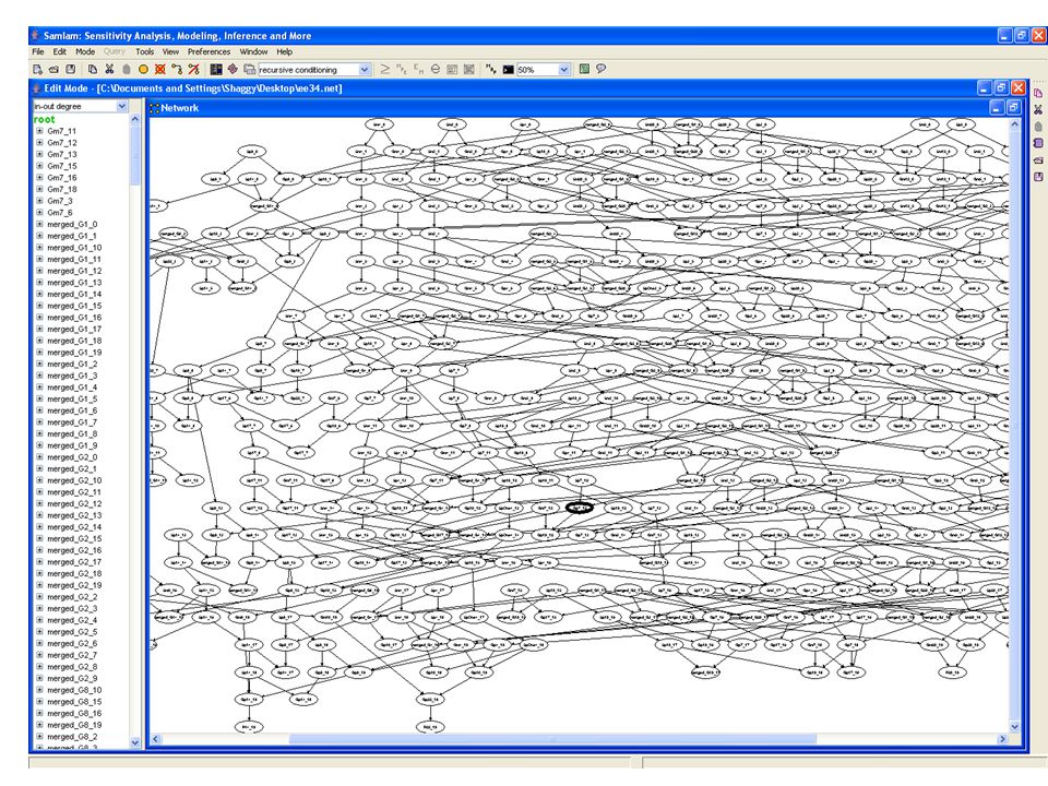
108. Arithmetic Circuit Gene 1 Gene 2

109. State of the Art Linkage PedigreeOffline (sec) AC EdgesOnline (sec) Superlink 1.4 (sec) EE3325.332,070,7070.591,046.72 EE3761.291,855,4100.391,381.61 EE30376.7827,997,6868.37815.33 EE2389.473,986,8161.08502.02 EE18283.9623,632,2006.63248.11

110. Model Compilation: Factoring MLFs into ACs Classical algorithms factor MLFs into ACs: Jointree embeds AC Variable elimination constructs AC bottom up Recursive conditioning constructs AC top down Factoring MLFs into ACs can be reduced to logical reasoning Exploiting local structure to build smaller ACs: Compiling models with very high treewidth is common place Boundary between exact and approximate inference is much changed Public systems now available!