Download presentation
Presentation is loading. Please wait.

1
Simulink Modelling Tutorial In Simulink, it is very straightforward to represent a physical system or a model. In general, a dynamic system can be constructed from just basic physical laws. We will demonstrate through some examples. We begin by demonstrating the train model as below

2
Train system The train consists of an engine and a car. We assume that the train only travels in one direction The mass of the engine and the car will be represented by M1 and M2, respectively. The two are held together by a spring with stiffness k. (F) is the force of the engine, (µ) represents the coefficient of rolling friction. We want to apply control to the train so that it has a smooth start-up and stop, along with a constant-speed ride.
 is the force of the engine, (µ) represents the coefficient of rolling friction. We want to apply control to the train so that it has a smooth start-up and stop, along with a constant-speed ride..")
3
Free body diagram and Newton's law The system can be represented by following Free Body Diagrams. By Newton's law: the sum of forces on a mass = the mass x acc’n

4
The Equations of Motion Sum(forces_on_M 1 )=M 1 *x 1 ” Or F – k(x 1 -x 2 ) - µ.M 1. g.x 1 ’= M 1.x 1 ” Or x 1 ” = 1/M 1 (F – k(x 1 -x 2 ) - µ.M 1. g.x 1 ’) The red represents the summation of all forces, hence we need to employ a summation box in Simulink and Sum(forces_on_M 2 )=M 2 *x 2 ” Or k(x 1 -x 2 ) - µ.M 2. g.x 2 ’= M 2.x 2 ’’ Or x 2 ” = 1/M 2 (k(x 1 -x 2 ) - µ.M 2. g.x 2 ’) The red represents the summation of all forces, hence we need to employ a summation box in Simulink
 - µ.M 1. g.x 1 ’) The red represents the summation of all forces, hence we need to employ a summation box in Simulink and Sum(forces_on_M 2 )=M 2 *x 2 Or k(x 1 -x 2 ) - µ.M 2. g.x 2 ’= M 2.x 2 ’’ Or x 2 = 1/M 2 (k(x 1 -x 2 ) - µ.M 2. g.x 2 ’) The red represents the summation of all forces, hence we need to employ a summation box in Simulink.")
5
Graphical Representations Open a new model window, and drag two Sum blocks (from the Linear library), one above the other. Label these: "Sum_F1" and "Sum_F2". The outputs of each of these Sum blocks represents the sum of the forces acting on each mass. Multiplying by 1/M will give the acceleration.

6
Add the Gains Drag two Gain blocks into your model and attach each one with a line to the outputs of the Sum blocks Double-click on the upper Gain block and enter 1/M1 Similarly, change the second Gain block to 1/M2

7
Enlarge each gain to show its expression Also, label these two Gain blocks "a1" and "a2".

8
Adding Integrators a1 & a2 are the accelerations Integrating the accel’n, gives the velocities (v1 & v2) Integrating v1 & v2 gives the disp’t (x1 & x2) So we add 4 integrator blocks 1/s and labels to blocks
 Integrating v1 & v2 gives the disp’t (x1 & x2) So we add 4 integrator blocks 1/s and labels to blocks")
9
Adding Scopes to view output Now, drag two Scopes from the Sinks library into your model and connect them to the outputs of these integrators. Label them "View_x1" and "View_x2".

10
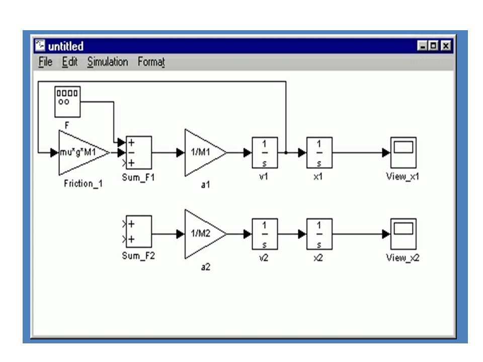
Adding the Forces Now we are ready to add in the forces acting on each mass. First, you need to adjust the inputs on each Sum block to represent the proper number of forces. There are a total of 3 forces acting on M1, so change the (Sum_F1) block's dialog box entry to: +++ There are only 2 forces acting on M2, so we can leave Sum_F1 alone for now
 block s dialog box entry to: +++ There are only 2 forces acting on M2, so we can leave Sum_F1 alone for now.")
11
The diagram now looks like this:

12
Adding the driving force (F) The first force acting on M1 is just the input force, F. Drag a Signal Generator block from the Sources library and connect it to the uppermost input of the (Sum_F1) block. Label the Signal Generator "F".
 block. Label the Signal Generator F ..")
13
Adding the friction force on M1 This force is equal to: µ*g*M1*v1 Tap off the velocity signal and multiply by a gain, (µ*g*M1). Drag a Gain block into your model window. and connect it to the v1 integrator Connect the output of the Gain block to the second input of (Sum_F1). Change the gain of this gain block to (µ*g*M1) Re-size and label the gain block (Friction_1). This force, however, acts in the negative x1-direction. So, it must come into the (Sum_F1) block with negative sign. Change the list of signs of (Sum_F1) to (+-+). The diagram now looks like:
. Change the gain of this gain block to (µ*g*M1) Re-size and label the gain block (Friction_1). This force, however, acts in the negative x1-direction. So, it must come into the (Sum_F1) block with negative sign. Change the list of signs of (Sum_F1) to (+-+). The diagram now looks like:.")
15
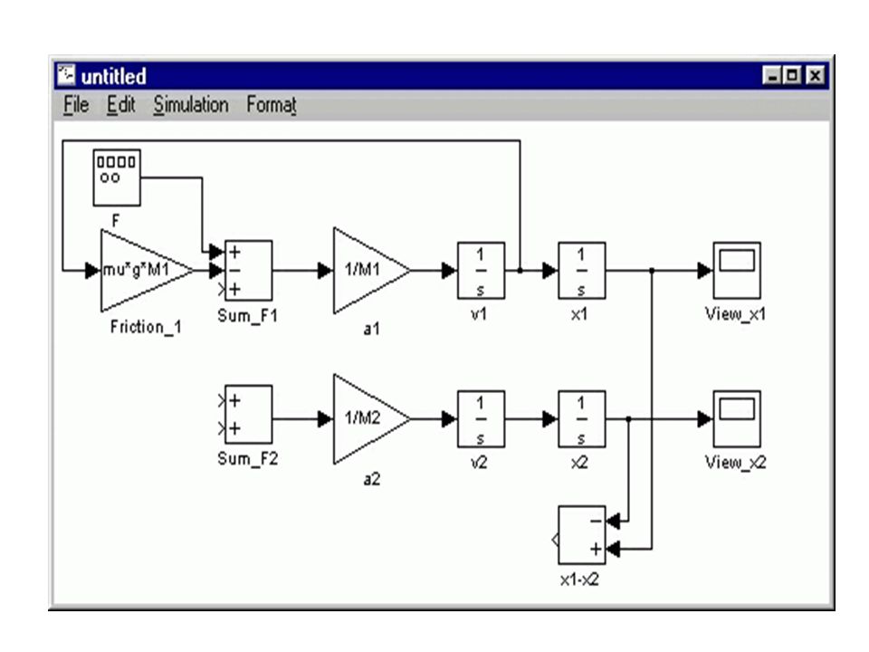
Adding the Spring Force The last force acting on M1 is the spring force between masses. This is equal to: k*(x1-x2) First, we need to generate (x1-x2) which we can then multiply by (k) to generate the force. Drag a Sum block below the rest of your model & label it "(x1-x2)" and change its list of signs to (-+) Since this summation comes from right to left, we need to flip the block around. Select the block by single- clicking on it and select Flip from the Format menu (or hit Ctrl-F). Now, tap off the x2 signal and connect it to the negative input of the (x1-x2) Sum block. Tap off the x1 signal and connect it to the positive input. You should see the following:
 First, we need to generate (x1-x2) which we can then multiply by (k) to generate the force. Drag a Sum block below the rest of your model & label it (x1-x2) and change its list of signs to (-+) Since this summation comes from right to left, we need to flip the block around. Select the block by single- clicking on it and select Flip from the Format menu (or hit Ctrl-F). Now, tap off the x2 signal and connect it to the negative input of the (x1-x2) Sum block. Tap off the x1 signal and connect it to the positive input. You should see the following:.")
17
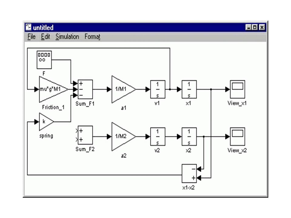
Continue adding the spring force Now, we multiply (x1-x2) by (k) to get the spring force. Drag a Gain block into your model to the left of the Sum blocks, change it's value to (k) and label it "spring". Connect the output of the (x1-x2) block to the input of the spring block, and the output of the spring block to the third input of (Sum_F1). Change the third sign of Sum_F1 to negative (use +--). Now the diagram looks like this:
 and label it spring . Connect the output of the (x1-x2) block to the input of the spring block, and the output of the spring block to the third input of (Sum_F1). Change the third sign of Sum_F1 to negative (use +--). Now the diagram looks like this:.")
19
Adding the spring force to M2 Now, we can apply forces to M2. For the first force, we will use the same spring force we just generated, except that it adds in with positive sign. Simply tap off the output of the spring block and connect it to the first input of Sum_F2.

20
Adding the Friction force on M2 The last force to add in the friction on M2. Tap off v2, multiplying by a gain of ( µ *g*M2) and add to (Sum_F2) with negative sign. We get the following:
 and add to (Sum_F2) with negative sign. We get the following:.")
21
Final Touches Now the model is complete. We simply need to supply the proper input and view the proper output. The input of the system will be the force, F, provided by the engine. We already have placed the function generator at the input. The output of the system will be the velocity of the engine. Drag a Scope block from the Sinks block library into your model. Tap a line off the output of the "v1" integrator block to view the output. Label the scope "View_v1".

22
Final Diagram The model is complete. Save your model.

23
Running the Model Before running the model, we need to assign numerical values to each of the variables used in the model. For the train system, let M1 = 1 kg M2 = 0.5 kg k = 1 N/sec F= 1 N u = 0.002 sec/m g = 9.8 m/s^2 Create an new m-file and enter the following commands. M1=1; M2=0.5; k=1; F=1; mu=0.002; g=9.8; Save and execute your m-file to define these values. Simulink will recognize MATLAB variables for use in the model.

24
Force Input for Engine Now, we need to give a suitable input to the engine. Double- click on the function generator (F block) and select a square wave with frequency.001Hz and amplitude -1 (positive amplitude steps, negative before stepping positive).
 and select a square wave with frequency.001Hz and amplitude -1 (positive amplitude steps, negative before stepping positive)..")
25
Decide on the Simulation Time The last step before running the simulation is to select a suitable simulation time. To view one cycle of the.001Hz square wave, we should simulate for 1000 seconds. Select Parameters from the Simulation menu and change the Stop Time field to 1000. Close the dialog box. Now, run the simulation and open the (View_v1) scope to examine the velocity output (hit auto-scale). The input was a square wave with two steps, one positive and one negative. Physically, this means the engine first went forward, then in reverse. The velocity output reflects this.
 scope to examine the velocity output (hit auto-scale). The input was a square wave with two steps, one positive and one negative. Physically, this means the engine first went forward, then in reverse. The velocity output reflects this..")
26
Velocity Output After running the simulation, we get the following trace for the velocity output:

Similar presentations


 T(t) (t) q(t) x(t)>")


 played a significant role in developing our idea of Force. He explained the link between force and.>")


