1. Chapter 2 Data Analysis

2. 2.1 Units of Measurement Before 1795, measurement units were inexact!!!!

3. 2.1 Units of Measurement In 1960 the metric system was updated and is called the Systeme Internationale d’Unites or the SI unit of measurement. Standard units of measurement for ALL scientists to use worldwide.

4. Base Unit - unit of measurement based on an object or event in the physical world The standard kilogram is stored in a vault at the International Bureau of Weights and Standards near Paris. It is made of a platinum-iridium alloy, and is shown here next to an inch-based ruler for scale.

5. Base Units: 2. Time: second (s) 3. Length: meter (m) 4. Mass: kilogram (kg)

6. 5. Temperature: Kelvin (K) 6. Amount of substance: mole (mol) an international standard to measure an "amount of stuff" aka Mole! It refers to the number of atoms in 12 grams of carbon 12 (6.022 x 10 23 ) Avagadro’s Number

7. Derived Unit - A unit that is a combination of base units. There are hundreds of units needed for measuring “everything,” but they are all derived from those base units.

8. 1.Volume = L x W x H for a regularly shaped solid cubic meter (m 3 ),cubic centimeter (cm 3 ) or cubic decimeter (dm 3 )  Unit for volume: liter (L) for a liquid  1 dm 3 = 1 L 1 cm 3 = 1 mL

9. 2.Density- ratio that compares the mass of an object to its volume  Units are grams per cubic centimeter (g/cm 3 )  1 ml = 1 cm 3

10.  density = mass volume  Density is a property that can be used to identify an unknown sample of matter.

11. Temperature Kelvin – SI base unit for temperature ºC + 273 = K K – 273 = ºC There are no negative temperatures in Kelvin

12. 2.2 Scientific Notation Scientific Notation- expresses numbers as a multiple of two factors: 1. A number between 1 and 10 2. Ten is raised to a power (exponent). 2.0 x 10 3  3 is the exponent 2.0 x 10 3 = 2000.20 or 20 would be WRONG because they are NOT numbers between 1 and 10!!

13. Scientific Notation Example Count the number of places the decimal point moved and the direction Convert 436289 to scientific notation. 1.Place decimal at end of number 436289. 2.Move decimal to place it behind the first number 4.36289 3.You moved the decimal 5 places left.  4.If decimal moves left, the exponent is positive 5.The # of times the decimal was moved becomes the exponent. 4.36289 x 10 5

14. –If decimal moves left, exponent is positive –if decimal moves right, exponent is negative

15. Convert.000872 to scientific notation 1.Move the decimal behind first number that is NOT a zero. 0008.72 2.8.72 You moved the decimal 4 places right.  3.The # of times the decimal was moved becomes the exponent. 4.If decimal moves right, exponent is negative. 5.The # of times the decimal was moved becomes the negative exponent  8.72 x 10 – 4

16. To convert Scientific Notation to Standard Notation Reverse the above steps: If the exponent is positive move the decimal to the right the same number of places as the exponent. 2.5 x 10 4 = 25 000 If the exponent is negative move the decimal to the left the same number of places as the exponent. 2.5 x 10 -4 =.00025

17. Adding, subtracting, multiplying, and dividing in Scientific Notation by using the calculator –Use “EE” or “exp” key on your calculator to replace “ x 10^” –Ex: 8.72 x 10 -4 would be 8.72”EE”-4

18. Dimensional Analysis - Conversion of one unit to another Conversion factor- ratio of equivalent values used to express the same quantity in different units Ex: 1 km = 1000 m

19. Convert 48 km to m. 1. Write starting value 48 km 2. Then, multiply by the conversion factor with the starting unit on bottom 48 km x 1000m 1 km 3. Multiply by number on top and divide by the one on the bottom. 4. Cancel the same units. = 48,000 m OR 4.8 x 10 4

20. Sect. 2.3: How reliable are measurements? Accuracy – how close a measured value is to an accepted or true value Precision – how close a series of measurements are to each other Compare to throwing darts bottom of pg 36.

22. ACCURACY VS. PRECISION: HOWEVER, if the actual time is 3:00, then the second clock is more accurate than the first one. ACCURACY = HOW CLOSE A MEASUREMENT IS TO THE TRUE VALUE PRECISION = EXACTNESS THIS CLOCK is more precise than THIS CLOCK

23. Percent error – the ratio of an error to an accepted value. % error = experimental – accepted x 100 accepted value Example: Density of lead is 11.3, you had 10.3 in your experiment. Difference is 1 So 1 x 100 = 8.8% 11.3

24. Significant Figures Accuracy is limited by the available tools. Sig figs are based on instrument precision (numbers can only be as exact as the instrument is) Instruments must be calibrated to assure accuracy.

25. The “best” number is the one with the most decimal places. So 3.54 g is MORE precise than 3.5 g. Significant figures - include all known digits plus ONE estimated digit.

26. Having Trouble with Sig Figs? Try this: 1. Determine if the decimal point is “present” or “absent”. 2. Picture a map of the U.S. with the Pacific Ocean on the left and the Atlantic Ocean on the right. PACIFICATLANTIC Decimal presentDecimal absent  3. If the decimal point is “present”, imagine an arrow LEFT from the Pacific Ocean pointing to the number. (Think “P” for “present” and “Pacific”).  4. If the decimal point is “absent”, imagine an arrow RIGHT from the Atlantic Ocean pointing to the number (“A” for “absent” and “Atlantic”).  5. Start counting digits when the arrow hits a non-zero digit. Each digit after that is significant.

27. EXAMPLES: .009120 has 4 sig figs (9 is the first non- zero digit counting from Pacific)  1.050 has 4 sig figs (1 is the first non- zero digit counting from Pacific) 34005  has 5 sig figs (5 is the first non- zero digit counting from Atlantic) 1200  has 2 sig figs (2 is the first non- zero digit counting from Atlantic)

28. Rounding Numbers If last number is five or greater, round up. 12.6 13 If last number is less than five, leave alone. 12.2 12

29. Rounding Examples 12.27845 Round to 3 significant figures 12.3 Round to 5 significant figures 12.278 Round to 4 significant figures 12.28 Round to 2 significant figures 12

30. Math with Sig Figs When adding/subtracting, answer will be rounded to least number of decimal places 28.0 cm 23.538 cm + 25.68 cm 77.218 cm so the answer must have only one digit to the right of the decimal 77.2 cm is the answer

31. When multiplying/dividing, answer will be rounded to least number of sig figs 3.20 cm x 3.65 cm x 2.05 cm = 23.944 cm 3 all the factors have 3 sig figs So the answer should have 3 sig figs 23.944 cm 3 Becomes 23.9 cm 3

32. Mult/Div Round to the least number of sig figs 2.50 m x 0.05 m x 5.00 m = 0.625 m 3 3 sig figs 1 sig fig 3 sig figs The answer should have one sig fig. The answer would be 0.6 m 3 (1200 cm. /. 3.0 cm). /. 400.0 cm = 1 cm 3 2 sig figs 2 sig fig 4 sig figs The answer should have 2 sig figs The answer would be 1.0 cm 3

33. Section 2.4: Representing Data A goal of many experiments is to discover whether a pattern exits. Data in a table may not show an obvious pattern. Graphing can help reveal a pattern.

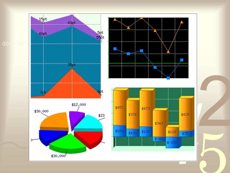
34. Graph – visual display of data 3 types of Graphs –Circle graph/pie chart –Bar Graph –Line Graph

36. HOW TO CHOOSE WHICH TYPE OF GRAPH TO USE? When to Use...... a Pie Chart. Pie charts are best to use when you are trying to compare parts of a whole. They do not show changes over time.

37. When to Use...... a Bar Graph. Bar graphs are used to show how a quantity changes with certain factors or to compare things between different groups or to track changes over time. Bar graphs are best when the changes are larger.

38. When to Use...... a Line graph. Line graphs are used to track changes over short and long periods of time. When smaller changes exist, line graphs are better to use than bar graphs. Line graphs can also be used to compare changes over the same period of time for more than one group.

39. DRY MIX Independent variable is graphed on the x-axis Dependent variable is graphed on the y-axis

40. Distance /Time Graph