1. 1 st semester 1436 / 1437

2. Modulation Continuous wave (CW) modulation AM Angle modulation FM PM Pulse Modulation Analog Pulse Modulation PAMPPMPDM Digital Pulse Modulation DMPCM

3. Introduction Continuous-wave(CW) modulation : a parameter of a sinusoidal carrier wave is varied continuously in accordance with the message signal. Amplitude Frequency Phase Pulse Modulation: signal is transmitted at discrete intervals of time. Pulse modulation can be analog pulse modulation or digital pulse modulation:

4. Introduction Analog pulse modulation: a periodic pulse train issued as a carrier and the following parameters of the pulse are modified in accordance with the corresponding sample value of the message signal. Pulse amplitude Pulse width Pulse position In the analog pulse modulation, information is transmitted basically in analog form, but the transmission takes place at discrete time

6. Introduction In digital pulse modulation, the message signal represented in a form that is discrete in both amplitude and time. The signal is transmitted as a sequence of coded pulses

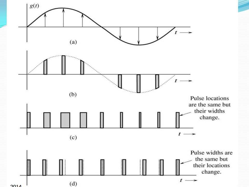
8. Pulse Amplitude Modulation (PAM) In the PAM, the amplitude of periodic pulse train is varied with a amplitude of the corresponding sample value of a continuous message signal. In PAM: width and position are fixed but amplitude varies

9. PAM

10. 10 PAM Natural PAM top portion of the pulses are subjected to follow the modulating wave. 1010/31/2012Punjab Edusat society

11. 11 PAM Flat topped PAM In this pulses have flat tops after modulation. 1110/31/2012Punjab Edusat society

12. Pulse Width Modulation (PWM) Pulse width modulation is also called pulse duration modulation (PDM). Pulse width modulation: position and amplitude are fixed but width varies PWM is more often used for control than for communication LEDs: output luminosity is proportional to average current.

13. PPM Pulse position modulation: width and amplitude are fixed but position varies The value of the signal determines the delay of the pulse from the clock

14. TDM In many cases, bandwidth of communication link is much greater than signal bandwidth. All three methods can be used with time-division multiplexing (TDM) to carry multiple signals over a single channel

15. Analog vs. Digital Communication Analog communication (baseband and modulated) is subject to noise. Analog Pulse modulations (PAM, PWM, PPM) represent analog signals by analog variations in pulses and are also subject to noise.

17. Digital Pulse Modulation The digital pulse modulation has two types:  Pulse Code Modulation(PCM)  Delta Modulation(DM) The process of Sampling which we have already discussed in initial slides is also adopted in digital pulse modulation

18. Pulse Code Modulation(PCM) PCM is the most basic form of digital pulse modulation. In PCM, a message signal is represented by a sequence of coded pulses, which is accomplished by representing the signal in discrete form in both time and amplitude. The basic operations performed in the transmitter of a PCM system are sampling, quantizing, and encoding.

19. The basic elements of a PCM system  Before we sample, we have to filter the signal to limit the maximum frequency of the signal as it affects the sampling rate.  Filtering should ensure that we do not distort the signal, i.e. remove high frequency components that affect the signal shape.

20. Sampler The sampler samples the input continuous-time analog signal at a sampling rate f s (= 1/T s sec). There are 3 sampling methods: Ideal - an impulse at each sampling instant Natural - a pulse of short width with varying amplitude Flattop - sample and hold, like natural but with single amplitude value

21. Quantization Process The analog signal has a continuous range of amplitudes and therefore its samples have a continuous amplitude range. In the quantization, the signal with continuous amplitude can be approximated by a signal constructed of discrete amplitudes selected on a minimum error basis from an available set.

22. Quantizer The sampling results is a series of pulses of varying amplitude values ranging between two limits: a min and a max. The amplitude values are infinite between the two limits. We need to map the infinite amplitude values onto a finite set of known values. This is achieved by dividing the distance between min and max into L zones, each of height   = (max - min)/L

23. Quantization Levels The midpoint of each zone is assigned a value from 0 to L-1 (resulting in L values) Each sample falling in a zone is then approximated to the value of the midpoint.

24. Quantization Zones Assume we have a voltage signal with amplitutes V min =-20V and V max =+20V. We want to use L=8 quantization levels. Zone width  = (20 - -20)/8 = 5 The 8 zones are: -20 to -15, -15 to -10, -10 to -5, -5 to 0, 0 to +5, +5 to +10, +10 to +15, +15 to +20 The midpoints are: -17.5, -12.5, -7.5, -2.5, 2.5, 7.5, 12.5, 17.5

25. Quantization Error When a signal is quantized, we introduce an error - the coded signal is an approximation of the actual amplitude value. The difference between actual and midpoint value is referred to as the quantization error. The more zones, the smaller  which results in smaller errors.

26. Encoding In combining the process of sampling and quantization, the specification of the continuous-time analog signal becomes limited to a discrete set of values. Representing each of this discrete set of values as a code called encoding process. Code consists of a number of code elements called symbols. In binary coding, the symbol take one of two distinct values. in ternary coding the symbol may be one of three distinct values and so on for the other codes.

27. Assigning Codes to Zones Each zone is assigned a binary code. The binary code consists of bits. The number of bits required to encode the zones, or the number of bits per sample, is obtained as follows: n b = log 2 L Given our example, n b = 3 The 8 zone (or level) codes are therefore: 000, 001, 010, 011, 100, 101, 110, and 111 Assigning codes to zones: 000 will refer to zone -20 to -15 001 to zone -15 to -10, etc.

28. Line Coding Any of several line codes can be used for the electrical representation of a binary data stream. Examples of line coding : RZ, NRZ, and Manchester

29. 2 10 t x(t) Consider the analog Signal x(t). 2 10 n X(nTs) The signal is first sampled Ts

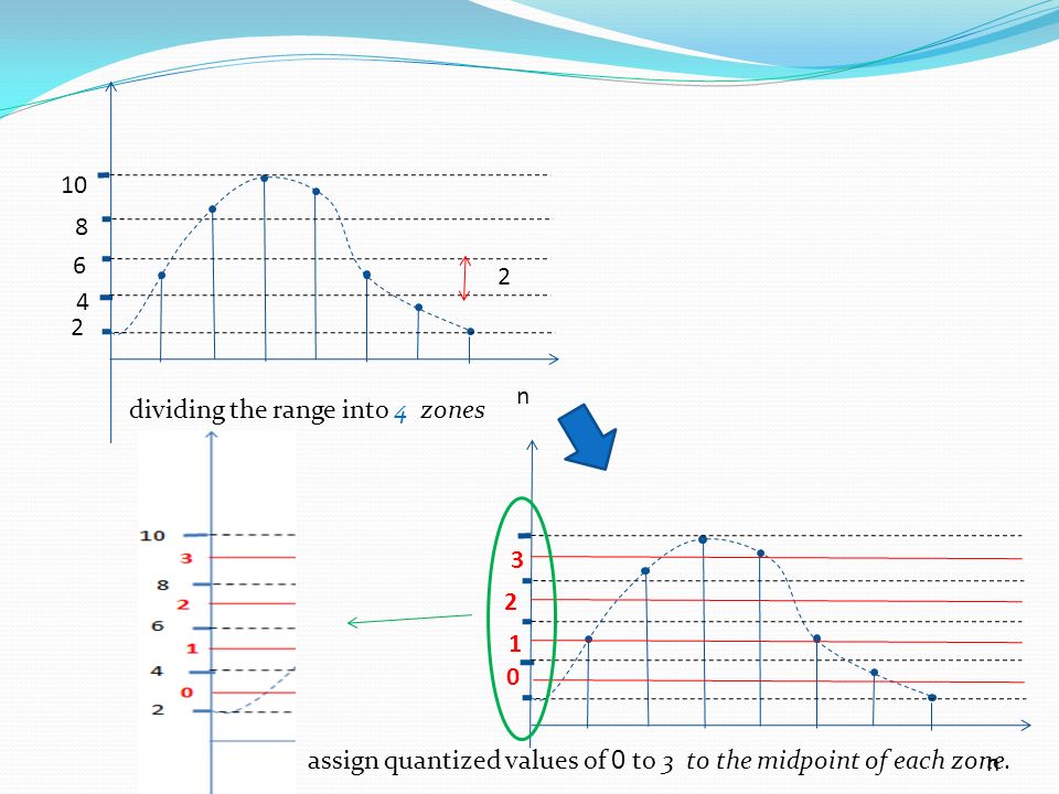
30. 2 4 6 8 n 10 2 dividing the range into 4 zones n assign quantized values of 0 to 3 to the midpoint of each zone. 0 1 2 3

31. n approximating the value of the sample amplitude to the quantized values. 0 1 2 3 n Each zone is assigned a binary code 0 1 2 3 00 01 10 11

32. n 0 1 2 3 00 01 10 11 00 01 11 The sequence bits if the samples 01111111010000 Use one of the line code scheme to get the digital signal