1. Chapters 5 and 6: Numerical Integration Code development trapezoid rule Simpson’s rule Gauss quadrature Laguerre quadrature Analysis changing the variable of integration estimating error in numerical integration uniform method to derive numerical integration

2. Derive the trapezoid rule

3. Usually x 1 = a and x n = b Replace f(x) on [a,b] by line p(x) Multiple intervals with f(x) on [x k-1,x k ] replaced by a line

4. Trapezoid rule: In-class work: Write a MatLab code for Trapezoid rule with arbitrary points where the integrand is evaluated. Input 2 arrays: x = values where the integrand is evaluated. f = values of the integrand at those points Output: trapezoid rule approximation to integral

5. Does your trapezoid rule code look something like function A=trap_arbitrary_points(x,f) n=length(x); sum=0; for k=2 to n sum=sum+(x k – x k-1 )(f k + f k-1 )/2; end A=sum; end

6. Write a script to apply trapezoid rule function to estimate with x k = exp(y k ) where y k =linspace(0,ln(5),10) What is the percent error in your result?

7. Does your script look something like inline definition of integrand y-vector defined by linspace(0,log(5),10) x-vector defined by exp(y) A = trap_arbitrary_points(x,integrand(x)) exact = result using anti-derivative percent difference=100abs((A-exact)/exact)

8. Expand your script to estimate with 10 equally spaced points between 1 and 5. What is the percent error in this result? How does it compare to your result with unequally spaced points where the integrand was evaluated?

9. Does your new script look something like inline definition of integrand y-vector defined by linspace(0,log(5),10) x-vector defined by exp(y) A1 = trap_arbitrary_points(x,integrand(x)) exact=result using anti-derivative percent difference1=100abs((A1-exact)/exact) x-vector defined by linspace(1,5,10) A2 = trap_arbitrary_points(x,integrand(x)) percent difference2=100abs((A2-exact)/exact) Which spacing gave a more accurate trapezoid-rule approximation?

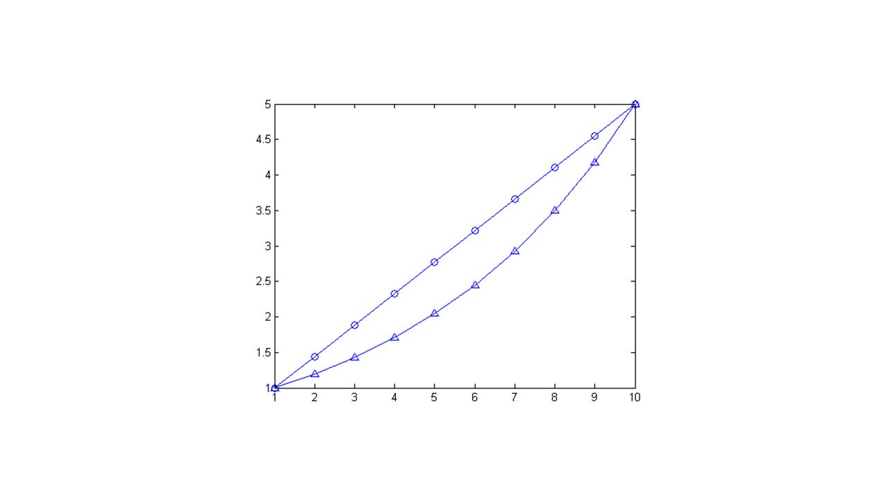
10. What is the difference between the two choices of where the integrand is evaluated? Display the 2 choices Plot the 2 choices What is your conclusion? Can you rationalize the difference in accuracy?

11. Does your new script look something like inline definition of integrand y-vector defined by linspace(0,log(5),10) x-vector defined by exp(y) A1 = trap_arbitrary_points(x,integrand(x)) exact=result using anti-derivative percent difference1=100abs((A1-exact)/exact) newx-vector defined by linspace(1,5,10) A2 = trap_arbitrary_points(newx,integrand(newx)) percent difference2=100abs((A2-exact)/exact) disp(x) disp(newx) plot(x,’^-’) plot(newx,’o-’)

13. Changing variable of integration

14. Use the transformation y = ln(x) to change the variable of integration. dy = dx/x x(y)= exp(y) Integrand is a function of y through x(y)

15. Expand your script to approximate x(y)= exp(y) using the integration variable y with 10 equally spaced points between 0 and ln(5)

16. Does your new script look something like inline definition of integrand y-vector defined by linspace(0,log(5),10) x-vector defined by exp(y) A1 = trap_arbitrary_points(x,integrand(x)) exact=result using anti-derivative percent difference1=100abs((A1-exact)/exact) x-vector defined by linspace(1,5,10) A2 = trap_arbitrary_points(x,integrand(x)) percent difference2=100abs((A2-exact)/exact) newx=exp(y) newintegrand=newx.*exp(-newx) A3 = trap_arbitrary_points(y,newintegrand) percent difference3=100abs((A3-exact)/exact) Which method of estimating the integral is most accurate?

17. In-class work last Thursday: Estimate the integral by the trapezoid rule with 10 points when the points are chosen in the following ways: 1. Equally spaced on [1, 5] 2. x k = exp(y k ) where y k = linspace(0,ln(5),10) 3. Equally spaced on [0, ln(5)] in the new integration variable y = ln(x). Calculate the percent difference from the exact value in each case Results for percent difference: (1) 1.6407, (2) 1.1756, (3) 0.0995

18. What we learned from in-class work last Thursday: 1. Concentrating sample points where integrand is large gives a slight improvement in accuracy over equally-spaced sample points. 2. A different integration variable may give a significant improvement in accuracy.

19. Assignment 5, Due 2/4/16 On page 242 of the text (6 th edition), the value of is given as -18.79829683678703, which can be taken as the “exact” value. Estimate this integral by the trapezoid rule with 10 points when the points are chosen in the following ways: 1. Equally spaced on [1, 3] 2. x k = exp(y k ) where y k = linspace(0,ln(3),10) 3. Equally spaced on [0, ln(3)] in the new integration variable y = ln(x). Calculate the percent difference from the exact value in each case

20. Accuracy increases with the number of points where the integrand is evaluated. More trapezoids means shorter bases. Line segments replacing the integrand are shorter and better able to follow changes in the integrand over the range of integration. With equally spaced sample points, the formula for trapezoid rule simplifies due to common width of base. Called the “composite” trapezoid rule Trapezoid Rule

21. When the integrand is replaced by a polynomial, the integral between a and b, can be done analytically if we know the coefficients of the polynomial. Given values of the integrand f(x) at n points we can determine a polynomial of degree n-1 that passes through those points. If we are given only f(a) and f(b) we can determine the equation of a line (degree=1) that passes through them.

22. Which is the same result that we got using the area of trapezoid 2

23. Use Taylor formula to derive an analytic expression for the error in the composite trapezoid rule as a function of the number of points where the integrand is evaluated.

24. Estimate error in Trap Rule: single subinterval of size h exact result but we don’t know the value of   a    a+h By fundamental theorem of calculous

25. Estimate error in Trap Rule: single subinterval of size h Difference between exact and trap rule Exact from previous slide Trap rule approximation a    a+h

26. Estimate error in Trap Rule: n subinterval of size h n is number of subinterval 1

27. by the composite trapezoid rule with 10 points  = (b-a) 3 |f “(  )|/12n 2 a<  <b but we don’t know its value Can’t get a value for f ”(  but we can bound |f “(  )|  < (b-a) 3 |f “(  )| max /12n 2 Plot |f “(x)| between a and b to fine its maximum value Remember! n is the number of subinterval In class work: Estimate the error in approximating

28. radians (by default) |sin(x)| fplot(‘abs(sin(x))’,[2,5])

29. by the composite trapezoid rule with 10 points Get the exact value by anti derivative Calculate trapezoid-rule estimate Actual error = abs(estimate-exact) In class work: What is the actual the error in approximating

30. by the composite trapezoid rule with an error less than 0.25x10 -4  = (b-a)h 2 |f “(  )|/12 < 0.25x10 -4 solve for h Same problem different form: estimate how small h must be to evaluate

31. by the composite trapezoid rule with 10 points  < (b-a) 3 |f “(  )| max /12n 2 Don’t forget the chain rule when you take the derivative Assignment 6, Due 2/9/16 Estimate the error in approximating

32. Does your plot of |f ’’(x)| look something like this? Under tools, select data cursor Is your estimate of upper bound on absolute error in trap-rule ~ 31.7? Compare to trap-rule result with 10 points. What does this tell you about your trap-rule estimate of the integral?

33. Plot of f(x) Would you expect trap-rule with 10 points to give a good result? Trap-rule with 10 points to give an idea about the “scale” of

34. If the scale of is ~ 0.2, then 0.002 might be a reasonable upper bound on absolute error in trap-rule approximation How many points are required to reduce the estimated upper bound on the trap-rule error to ~ 0.002? Better question: How small must h be to achieve this? Require  = (b-a)h 2 |f “(  )| max /12 < 0.002; solve for h Given h, find npts = 1+(b-a)/h Evaluate trap-rule with npts points 0.002 is what percent of your trap-rule estimate with npts?

35. Solution: h 2 < 12(0.002)/(6(142.6)) ~ 2.8x10 -5 h < 0.0053 npts > 1133.9 With 1134 points, the trap-rule approximation is 0.6385 The trap-rule approximation with 10 pts (-0.2309) was not acceptable, as expected from the upper bound of 31.7 on its absolute error. The scale of the trap-rule approximation with 10 pts is correct and provides enough information to design trap-rule approximation with high accuracy. MatLab’s numerical integration method, quad, returns a value 0.63845901. Absolute error in trap-rule with 1134 points is much less than the value of 0.002 that we required.

36. Problems from text on application of error formulas 5.1-6 p188 5.2-2 p 200 5.2-4 p200 5.2-7 p200 5.2-12 p210 6.1-2a p227 Numbers apply to 6 th addition

37. Most numerical integration formulas have the form Example: composite Trapezoid rule  0 =  n = 1/(2n)  k = 1/n if 1< k<n-1 n = number of subintervals One approach to deriving such formulas is to replace the integrand by polynomial of degree n

38. Lagrange interpolation formula is a way to replace integrand by a polynomial of degree n that is equal to the integrand at n+1 user-supplied points. See chapter 4 page 126 6 th edition 2 Review: Trapezoid rule derived by replacing integrand by line equal to integrand at 2 points

39. General formula for a polynomial of degree n that passes through a set of n+1 user-supplied point {x k,f(x k )}. p(x)

40. Example: derive Simpson’s rule

41. Simpson’s rule for one pair of subintervals

42. n pairs of subintervals

43. Pseudo code for Simpson’s rule A=function simprule(fh,a,b,npairs) h=(b-a)/2npairs sumeven=0 sumodd=0 for i=2,2,2npairs-2 sumeven end for i=1,2,2npairs-1 sumodd end A=h(fa+4sumodd+2sumeven+fb)/3

44. Assignment 7, Due 2/18/16 1. Approximate the integral 2. Use the Lagrange interpolation formula to derive a trapezoid rule approximation to the integral Using the value of the integrand –a and +a. Show that your result is the same as that derived from the area of a trapezoid? by the trapezoid and Simpson rules with 5 equally spaced points on [1,3]. Calculate the percent difference from the “exact” value, -18.79829683678703, in each case.

45. Error bound for composite Simpson’s rule |error| < (b-a)h 4 |f (4) (  )| max /180 a <  < b (text p221) h = width subintervals Since |error| proportional to |f (4) (  )|, Simpson’s rule is exact for a cubic, one degree higher than we should expect from a formula derived by replacing the integrand by a polynomial of degree 2. Test your CSR code on integral of x 3 from 0 to 2 with 5 points. Do you get the exact value?

46. Problem 6.1-4 text p228, 6 th ed Evaluated by composite Simpson’s rule with 5 points Bound the error. Compare to actual |error|. |error| = (b-a)h 4 |f (4) (  )|/180a <  < b (text p221) h = width subintervals

47. Problem 6.1-4 text p228, 6 th ed composite Simpson’s rule with 5 points = 0.693254 |exact-CSR| = 0.000107 |error| = (b-a)h 4 |f (4) (  )|/180a <  < b (text p221) h = width subintervals In this case, h = 0.25 f (4 ) (x) = 24/x 5 |f (4) (  )| < 24 1<  <2 |error| < (1)(0.25) 4 24/180 = 0.00052

48. by the CSR with an error less than 10 -4 Estimate the minimum number of points to evaluate |error| = (b-a)h 4 |f (4) (  )|/180a <  < b (text p221) h = width subintervals Hint: Find upper bound on h. Use to find a lower bound on pairs of subintervals. Use to find lower bound on number of points.

49. by the CSR with an error less than 10 -4 Estimate the minimum number of points to evaluate |error| = (b-a)h 4 |f (4) (  )|/180a <  < b (text p221) h = width subintervals h < 0.16549 npairs > 3.0213 npairs min = 4 npts = 2(npairs min ) + 1= 9

50. Simpson’s rule by simpler approach In each pair of subintervals of the CSR, we replace integrand by a polynomial of degree 2 that is equal to the integrand at 3 points. Lagrange interpolation formula gives us that polynomial without having to solve a 3x3 system of linear equations for the coefficients. We integrate the Lagrange polynomial over the pair of subintervals to get the weights in the Simpson’s rule approximation. An alternative and simpler approach is the develop a system of linear equations for the weights.

51. Find weights that give exact results for polynomials up to degree 2 Simpson’s rule with 1 pair of subintervals for range of integration [-a,a]

52. Problems from text p240 on deriving integration formulas 6.2-5 6.2-6 6.2-9 6.2-11

53. Assignment 8, Due 2/23/16 problem 6.2-6 text p240 Find A and B by requiring formula to be exact for f(x) = 1 and f(x) = x

54. Why is this not the Simpson’s rule?

55. Which is likely to be more accurate?

56. Review: Let {x 0, x 1, …, x n } be n+1 points on [a, b] where integrand evaluated, then numerical integration formula Will be exact for polynomials of degree at least n Trapezoid rule: (n = 1) exact for a line In general, error proportional to |f’’(  )| Simpson’s rule: (n = 2) exact for a cubic In general, error proportional to |f (4) (  )|

57. Gauss quadrature extents Simpson’s rule idea to its logical extreme: Give up all freedom about where the integrand will be evaluated to maximize the degree of polynomial for which formula is exact. nodes {x 0, x 1, …, x n } exist on [a, b] such that is exact for polynomials of degree at most 2n+1 Nodes are zeros of polynomial g(x) of degree n+1 defined by for 0 < k < n Gauss quadrature

58. Proof of Gauss quadrature theorem

59. For any set of n+1 nodes on [a,b]

60. Summary of Gauss Quadrature Theorem For any set of n+1 nodes on [a,b], is exact for polynomials up to degree n For the special set of node in Gauss quadrature, the formula is correct of polynomials of degree at most 2n+1 Nodes and weights, A i, depend on both [a,b] and n Scaling property of integrals lessens the impact of these dependences

61. Terms with odd powers of x in g(x) do not contribute due to symmetry Degree of g(x) = number of nodes Number of conditions on g(x) = number of nodes Number of conditions not Sufficient to determine all coefficients

62. Determines ratio of C 1 and C 3 only. As noted before, number of conditions on g(x) insufficient to determine all 4 coefficients of a cubic

63. Using plan (b) Compare with table 6.1, text p236

64. n = number of intervals Note symmetry of points and weights

65. Points and weights of Gauss quadrature are determined for Every integral from a to b can transformed into integral from -1 to 1

66. Nodes and weights determined for [-1,1] can be used for [a,b] Given values of y from table, this x(y) determines values on [a,b] where integrand will be evaluated

67. Example: Summary: Gauss quadrature n subintervals

68. with 2 nodes (no anti-derivative)

69. Pseudo-code GQ2345(a,b,f) % Gauss quadrature for integral of f between a and b with 2-5 points calculate points and weights by formulas in text p236 note symmetry calculate scale factor and coefficients in x(y) for each number of points calculate where in [a,b] integrand will be sampled calculate samples of integrand calculate weighted average of integrand samples multiply by scale factor return values

70. exact=2 quad=1.418302 Trap rule 800 =0.946803 Code and tests of 3 point Gauss quadrature

71. Assignment 9, Due 3/1/16: Make a table that includes the estimated value and percent difference (100|(exact-estimate)/exact| in approximated by the composite trapezoid rule, the composite Simpson’s rule and Gauss quadrature when the integrand is evaluated at 2, 3, 4, and 5 points, if possible. Hand in your MatLab codes. Quiz on numerical integration 3/8/16

72. More extensive tables of nodes and weights than given in text. Note that symmetry used to compress the table Verify that values for n = 2 to 5 are the same as n = 1 to 4 in table on P236 of text

73. Why is the integral hard to evaluate by numerical integration? Does the integral have a finite value? If so, can it be estimated by trapezoid rule, Simpson’s rule and Gauss quadrature?

74. Change the variable of integration in by the transformation y = ln(1/x) = -ln(x)

75. Change the variable of integration in y = ln(1/x) = -ln(x) when x=0 y=infinite when x=1 y=0 dy = -dx/x x(y) = exp(-y)

76. By arguments similar to the Guass-quadrature theorem, Laguerre derived an approximation to infinite integrals in which the integrand is evaluated at the zeroes of the Laguerre polynomials This formula only can be applied when f(x) is rapidly decreasing with increasing x

77. Note less symmetry than with Gauss quadrature Use first and last columns

78. Pseudo-code LQ2345(f) % Leguerre quadrature for integral between 0 and infinity with 2-5 points enter points and weights from table initialize sum for each number of points calculate integrand where it is be sampled calculate weighted average of integrand samples return values

79. Approximate integral in x variable by Guass quadrature with 2, 3, 4, and 5 points Approximate integral in y variable by Laguerre quadrature with 2, 3, 4, and 5 points Report your results as a table with approximate values and percent difference from exact. Assignment 10, Due 3/3/16:

80. Gauss with x as integration variable Laguerre with y = -ln(x) as integration variable