1. Mr. Patrick Caldwell Pacific Islands Liaison NOAA/NESDIS Data Centers August 27, 2009 Photo: Debbie and Kimbal Milikan

2. Talk Outline *Background and motivation *Validating historic surf observations *Translating observations *Empirical method to estimate surf *Surf-related coastal flood forecasts * Buoy spectral density composites (not time for all)

3. My Background: -Surfer in high school, 1970s (South Carolina) -Meteorology FSU,1984 -NOAA Data Center, UH Ocean. Dept, 1987 -Surf forecasting -Email 1993-1997 -Internet 1997 -NWS 2002-present Example of Email Forecast 1995 Background

4. November 9, 2002 Collaborative Surf Forecast is Born

5. Only Deep Water Swell Height, Period, and Direction No Surf Heights Surf Technical Advisory Group results: How to explicitly define surf height? How to translate deep water swell to surf heights? How to validate those heights?

6. Research Focus: North Shore - best available data Photo: A.Mozo Billabong XXL 2007

7. Data: Buoys and Visual Surf Observations Buoys Advantages: -Around the clock, high freq. samples -Wave spectrum Disadvantages in understanding surf -Data gaps -Not surf height

8. Historic Visual Surf Database, 1968-Present Primary visual reporting locations Goddard-Caldwell Dataset Wave Cams Daily Observations: - Surf News Network - Lifeguards -Coconut wireless - recent years: cams Database Caretaker Larry Goddard: 1968-1987 Pat Caldwell: 1987-present Daily value (upper-end of reported range (H1/10) for time of day of highest breakers) Recent years: Validation, Internet surf Pictures on web

9. Visual Surf Observations Pros: - explicitly quantify breaker size - inherent knowledge base - longest, most continuous (daily data since 8/1968) Cons: - subjectivity - only daylight, only few times/day - historically (often now) made in Hawaii scale Why surf observations are important? - validation - surf climatology - research (eg., empirical estimates) *most requested NODC dataset in Hawaii

10. Observations in history/science Hawaiian language: 135 words: moods of sea and surf 149 words: wind 87 words: rain 27 words: clouds Harold Kent, “Treasury of Hawaiian Words in 101 Categories”

11. Beaufort Wind Scale Developed in 1805 by Sir Francis Beaufort of England Visual observations to estimate wind speeds at sea on a scale of 1-12 Other Observations used In science: rogue waves

12. 2002- Hawaii Scale in the periscope!!!!!! Totally tasty tubes, brah

13. 1) Spatial variability Simulating Waves Nearshore (SWAN) Model Incident 2.5 m, 14 second from 315 o 315 o Incident 6.5 m, 19 second from 317 o 20m isobath Height (m) Understanding surf observations in terms of spatial and temporal surf height variability Until extra-large or higher! (Waimea the reporting spot) Surf observations made at zones of high refraction Simulating Waves Nearshore (SWAN) Model Caldwell, 2005, J.Coas.Res.

14. 2) Temporal variability What is the range given in surf reports? (if report given as X to Y (ocn Z), what does that mean?) 29 November, 2004 Waimea Buoy: 8’ 17 sec 325 deg: Aloha, this is GQ with your morning report, Sunset is 8-10 ocn 12 Photo courtesy: Merrifield/Millikan

15. Which heights occur more often? For heights of people filling a stadium, most would be centered closely around the average height, with far less people at the extreme short or tall level. Over a given time period, if every wave is sized and counted, most of the waves will be less than the average wave height. Most frequent Average height Significant height (H1/3) H1/10 H1/100 Wave height Count of people of each size 5’ 5.5’ 6’ 6.5’ height average Waves are different— Rayleigh Distribution Normal Distribution H 1/100 = 1.32 * H 1/10 H 1/3 = 0.79 * H 1/10 Count of waves of each size For Rayleigh distributions, one parameter can be calculated from another using simple multiplicative constants, for example, knowing the H1/10, one can calculate

16. 29 November, 2004 Benchmarks (surfers) Surf report: H1/3 to H1/10, ocn H1/100 With dominant energy 14-20 sec, roughly 4 waves per minute, or 100 waves in 25 minutes. Assume -waves in each set similar size - idealized 3 waves per set H1/3 : mean of highest 33, or 11 sets In 25 minutes, or one set every 2.5 min H1/10 : ave of highest 10, or 3 sets in 25 min or one set every 8.5 minutes H1/100 th : one set in 75 minutes highest 3 waves out of 300 waves (clean up or sneaker set) *waves are constantly arriving, however, reports were traditionally made by surfers for surfers who emphasize the smaller percentage of larger waves

17. Just as waves arrive in groups, or sets as surfers call it, there are also groups of groups, that is, spells (~0.5-2 hours) with much more frequent arrivals, and conversely, low energy time spans. Active arrival pattern Lull in arrivals Kilo Nalu Wave Sensor, offshore Honolulu during high southerly swell episode

18. Is Hawaii scale non-scientific (ie, inconsistent?) All Visual Surf Observations: -Course resolution -Hour to hour variability -Error increases with size -Research shows tendency to underestimate surf heights

19. What makes a dataset valid? Consistency Data Criteria -Oct-March -light winds -daylight hrs Buoy-Estimate -Assumes no loss of energy due to bottom friction -No refraction *only a proxy (test value) -Daylight maximum (assume 10 hr travel time) Caldwell, 2005, J.Coas.Res.

20. Validation of North Shore Surf Observations Surf Observation minus Buoy-estimated Surf Height Surf observations are temporally consistent Ratio = Difference / Estimated Height Caldwell, 2005, J.Coas.Res.

21. Another show of confidence in the GC dataset- high correlation to the buoy-estimated surf height Difference shows a quasi-normal distribution Caldwell, 2005, J.Coas.Res.

22. Three-way Comparisons: Buoy 51001, Waimea Buoy, and GC Observations (directionally filtered-- NW and NNW only) Kauai shadowing of WNW component High correlation among the three datasets— gives more confidence in GC database

23. Error Estimates Magnitude of Error increases with height Average Error ~15% Caldwell, 2005, J.Coas.Res.

24. North Shore Oahu Surf Climatology Caldwell, 2005, Validity of North Shore Surf Observations, Journal Coastal Res.

25. North Shore Surf Direction Climatology Caldwell, 2005, JCR No. Days Per Month (> 2 Hsf)

26. Surf Climatology Caldwell, 2005, JCR

27. 5’ Photo: C.Ferrari Sunset, November 22, 2002, Hsf=8 Translation from Hawaii Scale to Trough-to-Crest Heights Value recorded in the Goddard-Caldwell database The trough-to-crest surf height is defined as the vertical distance between the crest and the preceding trough at the moment and location along the wave front of highest cresting. For zones of high refraction with A-shaped peaks, the height refers to the center of the “A”. Errors: - trough identification ~ 10% of height - five-feet unit ~ +/- 6 inches or 10% of height Next Project: Presented: Wave Workshop Turtle Bay, Nov. 2004 Method: Photographic Evidence

28. Translation is a factor of two For the full range of breaker sizes Encountered in Hawaii within the 10-20% margin of error. This assumes the height is defined as the vertical distance between the crest and the preceding trough at the moment and location along the wave front of highest cresting and zones of high refraction (outer reefs) are included for extreme days when Waimea Bay was the reporting location. Caldwell and Aucan 2007, J.Coas.Res.

29. Photo:Jamie Ballenger Waimea, Jan. 25, 2003, HSF=25 The Waimea Curveball: translation Hawaii scale to Face changes Historic Database from zones of highest refraction until Sunset Beach is too large (~15 Hawaii scale). For days of heights >= 15 Hawaii scale, Waimea was/is the reporting location. However, under such conditions, this is no longer a zone of maximum refraction.

30. Study Area Waimea buoy Caldwell and Aucan 2007, J.Coas.Res.

31. 5’ Photo: C.Ferrari Waimea, January 10, 2004 Case Study: Three Sites, Same Day Assume H1/10 th (chose photographs with higher heights)

32. 5’ Photo: Hankfotos.com, Surfer: K.Bradshaw Outside Logs, January 10, 2004 Hank verified “H1/10 th ”, not clean-up set

33. 5’ Photo: E.Aeder Surfer: P.Cabrina, Note: Billabong XXL 2004 winner, as 70’ Peahi (Jaws), January 10, 2004 This likely H1/100 “Sneaker Set” **Result: 1968- visual surf observations translated to peak face, for extra-large days, refers to zones of high refraction on outer reefs

34. Deep water significant wave height does not mirror energy flux at shore– need at least dominant wave period or ideally directional spectra Kailua, January 27, 2008, photo: P.Caldwell Project: Estimate surf from deep water data/predictions

36. January 19, 2008, Sunset Beach Waimea buoy: 7’, 15 sec Photo: Alan Mozo

37. Empirical Method: Data: - Daily Surf Observations (HSF * 2) - Waimea Buoy maximum between 7am-5pm * Conservation of energy flux * Ignores refraction, diffraction, bottom friction, currents, wave-wave interactions, and wind Following Komar and Gaughan, 1973 Days removed from data: - strong trades - moderate or stronger onshore winds - 10 o < wave direction < 270 o

38. K r (H b ) = -0.003*H b 3 + 0.0099*H b 2 - 0.0250*H b + 1.0747 H surf = H b * K r (H b ) K r : coefficient of refraction H b : shoaling only estimator H surf : estimated surf height (shoaling + refraction) Caldwell and Aucan 2007, J.Coas.Res.

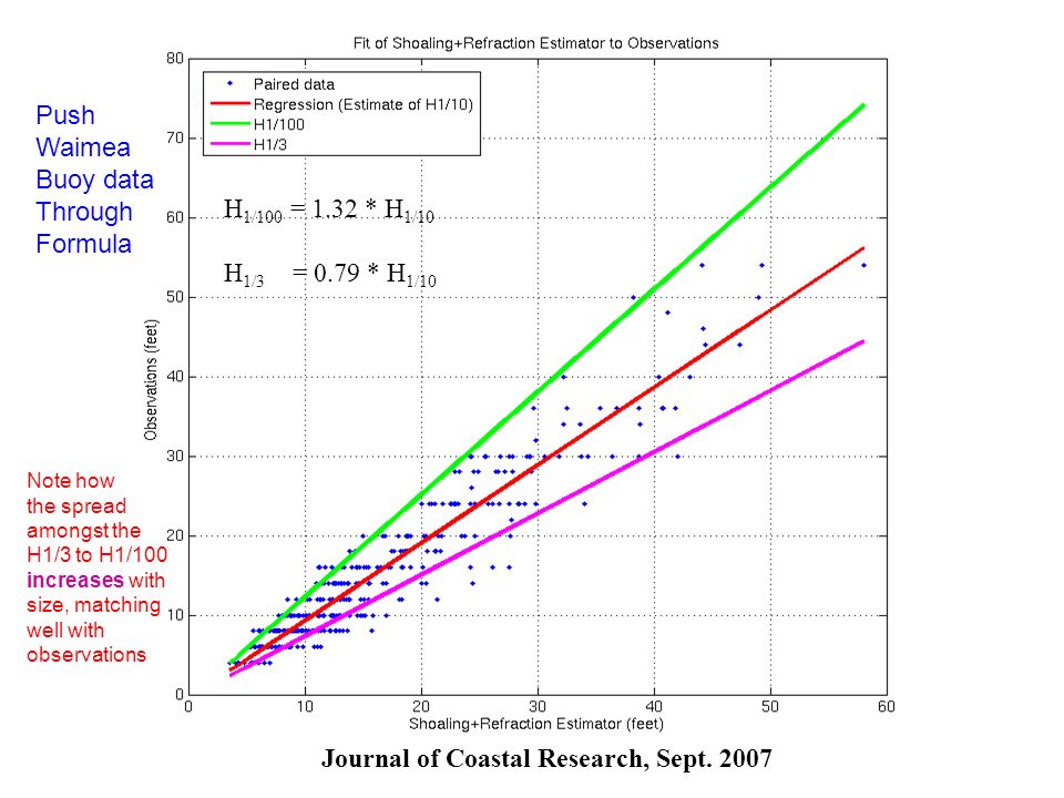
39. H 1/100 = 1.32 * H 1/10 H 1/3 = 0.79 * H 1/10 Push Waimea Buoy data Through Formula Note how the spread amongst the H1/3 to H1/100 increases with size, matching well with observations Journal of Coastal Research, Sept. 2007

40. NWS High surf advisory NWS High surf warning Weakness: 1)Short- period (windswell correction adapted) 2) Extreme surf (few validation points) 3) Wide spectra – overcalls it, break energy Into separate bands

41. Motivation Historical Context For Understanding Wave Run-up Journal of Coastal Research May 2009 Coinciding High Surf/Tides North Shore, Oahu Photo: Dolan Eversole, DLNR High Wave Run-up from Winter Extratropical Cyclones Jan 30, 2007

42. Wave Runup Issues: Safety!

44. December 1-4, 1969 Back-to-back giant surf episodes ($1500K 1970 dollars) Neap tides! Property Protection

45. Overview: Methodology Data Waves: 51001, Waimea Tides: Haleiwa and Kaneohe Procedure Correct 51001 Hs to Waimea Calculate hourly surf height Compare surf to tides, sort by category Derive recurrence, duration, joint probability Caldwell et. al. 2009, J.Coas.Res.

46. Example: Haleiwa Predicted Tides 2007 *Categories of tidal level based on standard deviations Heights above 1, 1.5, and 2 σ occur 15.6, 7.2, and 2.5% of the time Caldwell et. al. 2009, J.Coas.Res.

47. Semi-diurnal mixed tide Caldwell et. al. 2009, J.Coas.Res.

48. H s : 51001 versus Waimea Buoy Why 51001 > Waimea? -Closer to source * attentuation from dispersion greater closer to source * big surf episodes in Hawaii, source closer, so difference greater -Shadowing Niihau/Kauai Caldwell et. al. 2009, J.Coas.Res.

49. Results Caldwell et. al. 2009, J.Coas.Res.

50. Results -Decrease in occurrence as surf height and tide increase -Hawaii scale used as basis for surf height categories *essential for validation *based on bench marks *temporally consistent (Caldwell, JCR, 2005)

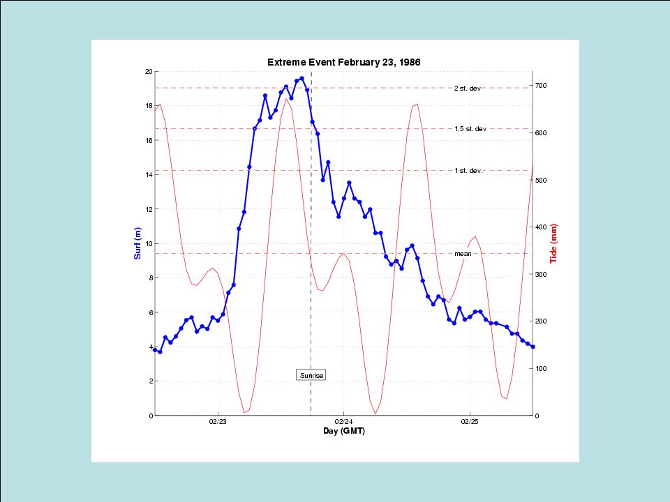
51. Case Study: February 23, 1986

54. 1 σ1.5 σ2 σ 15 Hsf 20 Hsf 25 Hsf 30 Hsf 10 Hsf suspicious data + C.Kontoes: Dept. of Transportation, NWS Storm Data No sand Lanis Sand Lanis Other Validation 1/13/2008, 7:10 am, buoy ~ 28 Hsf tide ~ 1.24 σ (HNL sea level anomaly 1/08 2.2cm) 1/30/2007 1:22am, buoy ~ 27 Hsf tide ~ 1.73 σ (HNL sea level anomaly 1/07: 3.9 cm) Photo: PC 9:45am Photo: D.Eversole, ~8am

55. 1 σ1.5 σ2 σ 15 Hsf 20 Hsf 25 Hsf 30 Hsf 10 Hsf suspicious data + C.Kontoes: Dept. of Transportation, NWS Storm Data No sand Lanis Sand Lanis Marginal Significant Extreme Nominal Categorizing 12/04/2007 12/07/2006

56. Joint Probability Model Caldwell et. al. 2009, J.Coas.Res. Contours are annual average number of hours Note widespread nature of extremes Exceedence distribution is one minus cumulative distribution Assume Hs and tides independent

57. Photo: Patrick Holzman -Surf information vital for … *protection of life and property *understanding near shore processes - beach dynamics - ecosystem variability - engineering - coastal planning