1. GOES-R 3 : Coastal CO 2 fluxes Pete Strutton, Burke Hales & Ricardo Letelier College of Oceanic and Atmospheric Sciences Oregon State University 1. The coastal ocean as a CO 2 sink (?) 2. Magnitude and variability of fluxes 3. Measurements during field work phase

2. Coastal CO 2 Fluxes pCO 2 in upwelling systems (coastal & equatorial) is associated with characteristic chlorophyll and SST signatures. Using techniques such as multiple linear regression, we can determine sea surface pCO 2 from space. Combining this with winds from either scatterometer(s) or coastal/buoy meteorological stations permits flux calculations. Important: In many areas we don’t even know the sign of the flux. Coastal ocean important for quantifying terrestrial fluxes.

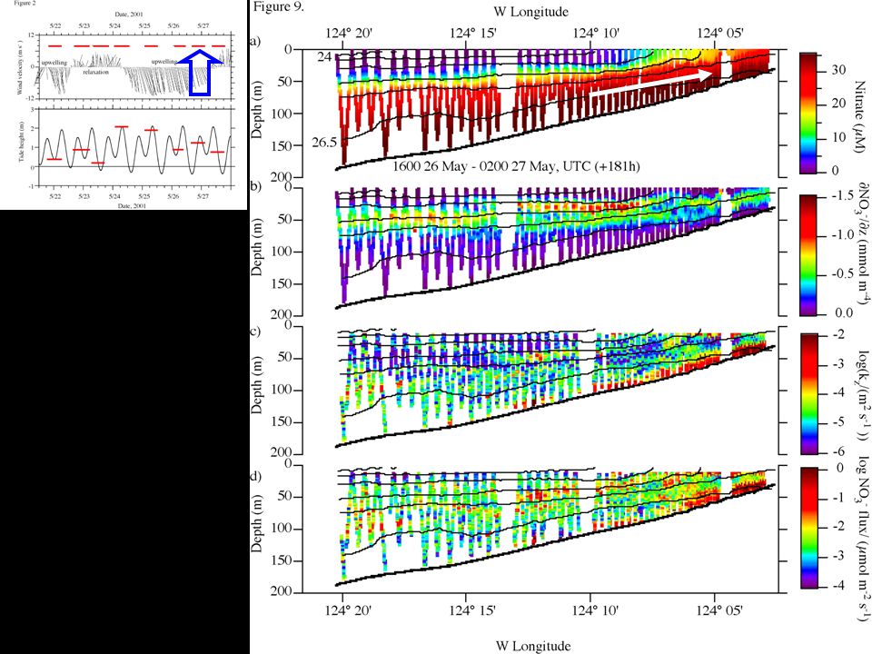
5. NO 3 NO 3 gradient Turbulent eddy-diffusion NO 3 flux

11. Coastal CO 2 : Relationship to temperature and chlorophyll Productivity & CO 2 uptake N limitation offshore

12. Coastal CO 2 : Relationship to temperature and POC

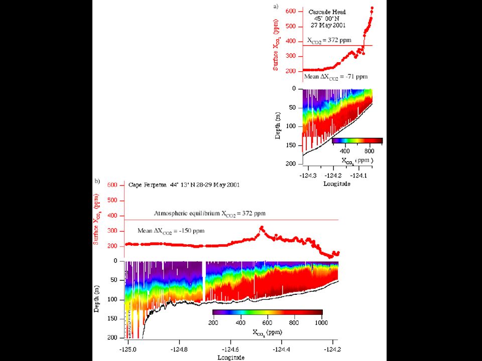
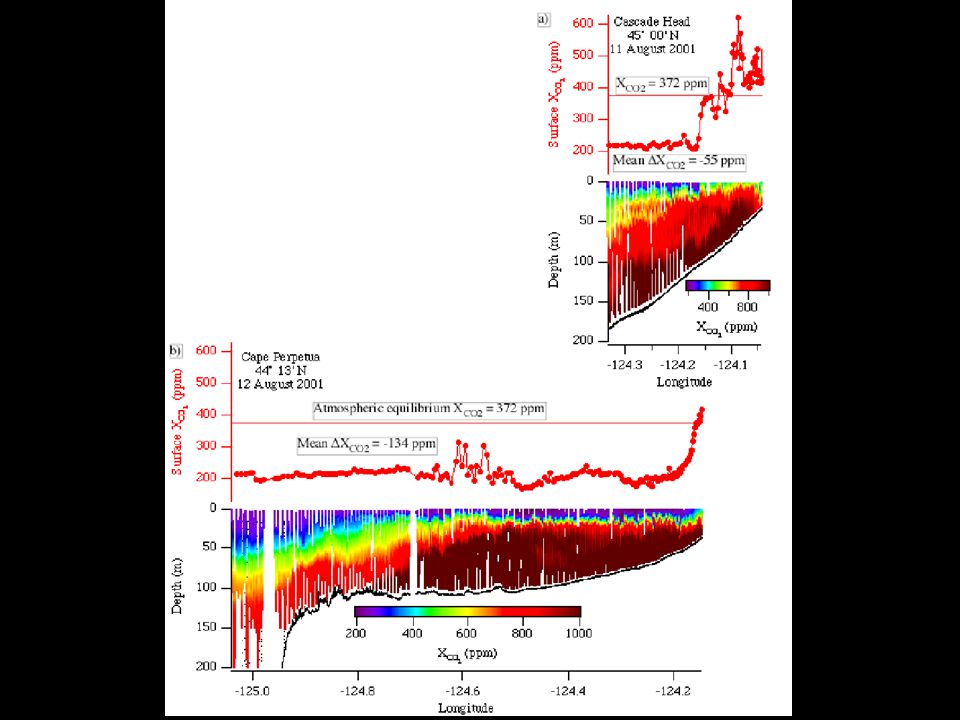
13. Characteristics of the Oregon upwelling system What makes this region a CO 2 sink? Strong (but episodic) upwelling throughout summer. Extremely rapid depletion of NO 3 and CO 2. –NO 3 depleted from ~34  M to essentially zero over ~10km –Corresponding drawdown of CO 2 from ~600 to 200ppm –Low concentrations offshore persist, despite variability nearshore –Mean along-transect CO 2 concentration typically ~300ppm –Implies  CO 2 ~70ppm (as much as 150ppm on some transects) Minimal warming of the upwelled waters ( cf California?) Keep these properties in mind for field work

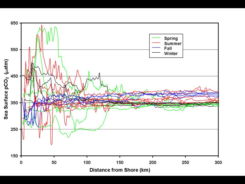
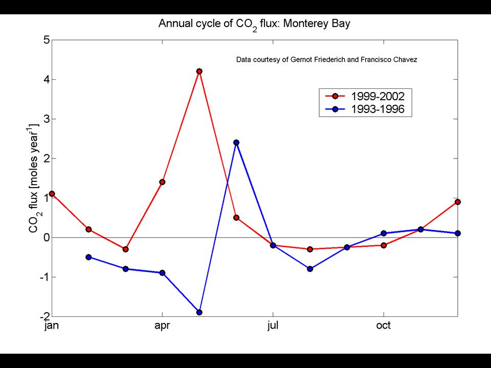
15. Characteristics of the California upwelling system In contrast to Oregon, not a strong source or sink. Possible reasons ( ie differences from Oregon) –Limitation of CO 2 drawdown by something other than NO 3 –Greater warming (works against biological uptake) Evidence for a significant change, towards a source, circa 1998 Illustrates the level of (lack of) understanding of the spatial and temporal variability.

16. Coastal CO 2 Fluxes: Satellite requirements Chlorophyll and SST will enable significant progress via multiple linear regression techniques. Temporal resolution ~3 hours will enable (primitive) budgets to be calculated: tracking of processes such as productivity and subduction. Higher temporal resolution of course better. This is a dynamic environment – any ability to ‘clear’ or alias clouds will enhance badly-needed coverage. Critical spatial scales ~1 to 10km. Current and proposed observational programs will provide the necessary in situ data for validation.

17. Field work: Underway measurements pCO2 Optics: ac9 (chl and POC), chl and CDOM fluorescence Physics: SST, salinity, winds for flux calculations Nutrients: Help interpret the drawdown story, particularly important for the MB experiment (NO 3 vs Fe limitation) Include wind data from coastal stations, buoys and scatterometer for comparison and estimates of spatial/temporal variability Consider the longer time scales: Frame our time window there within the year's upwelling dynamics

18. Field work: Sampling plan Repeated, long transects of all parameters Sub-km spatial resolution from very near shore, then offshore to where CO 2 and NO 3 stabilize existing data suggest ~150km at most for Monterey Bay Ideal: Uninterrupted transect work out (15+ hours) station work on the way back in Quantify spatial/temporal variability of the on-to-offshore gradient Do this ~5 times during the experiment, under different types of upwelling conditions Repeated aircraft overflights along the same track but at higher repetition would fill in the blanks.

19. Data analysis and interpretation Correlation (and other tools) to determine the relationship between pCO 2 and the measured optical/physical properties Quantification of the rates of warming and CO 2 drawdown from on- to off-shore Quantification of the spatial and temporal variability using data from repeated transects Use higher spatial and temporal resolution overflights to quantify precision/accuracy as a function of sampling Use this to justify our goals for spatial/temporal sampling

22. Coastal CO 2 : Relationship to physics and biology Productivity & CO 2 uptake N limitation offshore

23. What is the magnitude of the sink? Assume the conditions off Oregon are characteristic of upwelling regions along the entire west coast. Assume an upwelling season from May to August. Carbon sink is ~0.02 Pg C, approx. 5% of the annual mean North Pacific sink. …or ½ of the North Pacific sink for the same time period ( ie May to August).