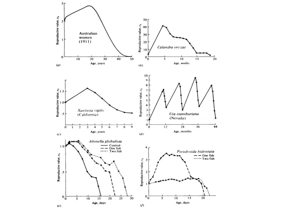
1. Life tables Age-specific probability statistics Force of mortality q x Survivorship l x Fecundity m x Realized fecundity l x m x Net reproductive rate R 0 Generation time T Reproductive value v x

2. v x = m x +  (l t / l x ) m t Residual reproductive value = age-specific expectation of offspring in distant future v x * = l x+1 / l x ) v x+1

3. Illustration of Calculation of E x, T, R 0, and v x in a Stable Population with Discrete Age Classes _____________________________________________________________________ AgeExpectation Reproductive Weighted of Life Value Survivor-Realizedby Realized E x v x Age (x) shipFecundityFecundityFecundity l x m x l x m x x l x m x _____________________________________________________________________ 0 1.0 0.0 0.00 0.00 3.40 1.00 1 0.8 0.2 0.16 0.16 3.00 1.25 2 0.6 0.3 0.18 0.36 2.67 1.40 3 0.4 1.0 0.40 1.20 2.50 1.65 4 0.4 0.6 0.24 0.96 1.50 0.65 5 0.2 0.1 0.02 0.10 1.00 0.10 6 0.0 0.0 0.00 0.00 0.00 0.00 Sums2.2 (GRR) 1.00 (R 0 ) 2.78 (T) _____________________________________________________________________ E 0 = (l 0 + l 1 + l 2 + l 3 + l 4 + l 5 )/l 0 = (1.0 + 0.8 + 0.6 + 0.4 + 0.4 + 0.2) / 1.0 = 3.4 / 1.0 E 1 = (l 1 + l 2 + l 3 + l 4 + l 5 )/l 1 = (0.8 + 0.6 + 0.4 + 0.4 + 0.2) / 0.8 = 2.4 / 0.8 = 3.0 E 2 = (l 2 + l 3 + l 4 + l 5 )/l 2 = (0.6 + 0.4 + 0.4 + 0.2) / 0.6 = 1.6 / 0.6 = 2.67 E 3 = (l 3 + l 4 + l 5 )/l 3 = (0.4 + 0.4 + 0.2) /0.4 = 1.0 / 0.4 = 2.5 E 4 = (l 4 + l 5 )/l 4 = (0.4 + 0.2) /0.4 = 0.6 / 0.4 = 1.5 E 5 = (l 5 ) /l 5 = 0.2 /0.2 = 1.0 v 1 = (l 1 /l 1 )m 1 +(l 2 /l 1 )m 2 +(l 3 /l 1 )m 3 +(l 4 /l 1 )m 4 +(l 5 /l 1 )m 5 = 0.2+0.225+0.50+0.3+0.025 = 1.25 v 2 = (l 2 /l 2 )m 2 + (l 3 /l 2 )m 3 + (l 4 /l 2 )m 4 + (l 5 /l 2 )m 5 = 0.30+0.67+0.40+ 0.03 = 1.40 v 3 = (l 3 /l 3 )m 3 + (l 4 /l 3 )m 4 + (l 5 /l 3 )m 5 = 1.0 + 0.6 + 0.05 = 1.65 v 4 = (l 4 /l 4 )m 4 + (l 5 /l 4 )m 5 = 0.60 + 0.05 = 0.65 v 5 = (l 5 /l 5 )m 5 = 0.1 ___________________________________________________________________________

4. Illustration of Calculation of E x, T, R 0, and v x in a Stable Population with Discrete Age Classes _____________________________________________________________________ AgeExpectation Reproductive Weighted of Life Value Survivor-Realizedby Realized E x v x Age (x) shipFecundityFecundityFecundity l x m x l x m x x l x m x _____________________________________________________________________ 0 1.0 0.0 0.00 0.00 3.40 1.00 1 0.8 0.2 0.16 0.16 3.00 1.25 2 0.6 0.3 0.18 0.36 2.67 1.40 3 0.4 1.0 0.40 1.20 2.50 1.65 4 0.4 0.6 0.24 0.96 1.50 0.65 5 0.2 0.1 0.02 0.10 1.00 0.10 6 0.0 0.0 0.00 0.00 0.00 0.00 Sums2.2 (GRR) 1.00 (R 0 ) 2.78 (T) _____________________________________________________________________ E 0 = (l 0 + l 1 + l 2 + l 3 + l 4 + l 5 )/l 0 = (1.0 + 0.8 + 0.6 + 0.4 + 0.4 + 0.2) / 1.0 = 3.4 / 1.0 E 1 = (l 1 + l 2 + l 3 + l 4 + l 5 )/l 1 = (0.8 + 0.6 + 0.4 + 0.4 + 0.2) / 0.8 = 2.4 / 0.8 = 3.0 E 2 = (l 2 + l 3 + l 4 + l 5 )/l 2 = (0.6 + 0.4 + 0.4 + 0.2) / 0.6 = 1.6 / 0.6 = 2.67 E 3 = (l 3 + l 4 + l 5 )/l 3 = (error: extra terms) 0.4 + 0.4 + 0.2) /0.4 = 1.0 / 0.4 = 2.5 E 4 = (l 4 + l 5 )/l 4 = (error: extra terms) 0.4 + 0.2) /0.4 = 0.6 / 0.4 = 1.5 E 5 = (l 5 ) /l 5 = 0.2 /0.2 = 1.0 v 1 = (l 1 /l 1 )m 1 +(l 2 /l 1 )m 2 +(l 3 /l 1 )m 3 +(l 4 /l 1 )m 4 +(l 5 /l 1 )m 5 = 0.2+0.225+0.50+0.3+0.025 = 1.25 v 2 = (l 2 /l 2 )m 2 + (l 3 /l 2 )m 3 + (l 4 /l 2 )m 4 + (l 5 /l 2 )m 5 = 0.30+0.67+0.40+ 0.03 = 1.40 v 3 = (l 3 /l 3 )m 3 + (l 4 /l 3 )m 4 + (l 5 /l 3 )m 5 = 1.0 + 0.6 + 0.05 = 1.65 v 4 = (l 4 /l 4 )m 4 + (l 5 /l 4 )m 5 = 0.60 + 0.05 = 0.65 v 5 = (l 5 /l 5 )m 5 = 0.1 ___________________________________________________________________________

6. Stable age distribution Stationary age distribution

7. Intrinsic rate of natural increase r = b – d when birth rate exceeds death rate (b > d), r is positive when death rate exceeds birth rate (d > b), r is negative Euler’s implicit equation:  e -rx l x m x = 1 (solved by iteration) If the net reproductive rate R 0 is near one, r ≈ log e R 0 /T

8. When R 0 equals one, r is zero When R 0 is greater than one, r is positive When R 0 is less than one, r is negative Maximal rate of natural increase, r max

9. Estimated Maximal Instantaneous Rates of Increase (r max, Per Capita Per Day) and Mean Generation Times ( in Days) for a Variety of Organisms ___________________________________________________________________ TaxonSpecies r max Generation Time (T) ----------------------------------------------------------------------------------------------------- BacteriumEscherichia coli ca. 60.00.014 ProtozoaParamecium aurelia1.24 0.33–0.50 ProtozoaParamecium caudatum0.94 0.10–0.50 InsectTribolium confusum 0.120 ca. 80 InsectCalandra oryzae0.110(.08–.11) 58 InsectRhizopertha dominica0.085(.07–.10) ca. 100 InsectPtinus tectus0.057102 InsectGibbum psylloides0.034129 InsectTrigonogenius globulosus0.032119 InsectStethomezium squamosum0.025147 InsectMezium affine0.022183 InsectPtinus fur0.014179 InsectEurostus hilleri0.010110 InsectPtinus sexpunctatus0.006215 InsectNiptus hololeucus0.006154 MammalRattus norwegicus0.015150 MammalMicrotus aggrestis0.013171 MammalCanis domesticus0.009 ca. 1000 InsectMagicicada septendcim0.001 6050 MammalHomo sapiens0.0003 ca. 7000 __________________________________________________________________ _

10. J - shaped exponential population growth

11. Instantaneous rate of change of N at time t is total births minus total deaths dN/dt = bN – dN = (b – d )N = rN N t = N 0 e rt log N t = log N 0 + log e rt = log N 0 + rt log R 0 = log 1 + rt r = log or = e r

12. Demographic and Environmental Stochasticity random walks, especially important in small populations Evolution of Reproductive Tactics Semelparous versus Interoparous Big Bang versus Repeated Reproduction Reproductive Effort (parental investment) Age of First Reproduction, alpha,  Age of Last Reproduction, omega, 

13. Mola mola (“Ocean Sunfish”) 200 million eggs! Poppy (Papaver rhoeas) produces only 4 seeds when stressed, but as many as 330,000 under ideal conditions

15. How much should an organism invest in any given act of reproduction? R. A. Fisher (1930) anticipated this question long ago: ‘It would be instructive to know not only by what physiological mechanism a just apportionment is made between the nutriment devoted to the gonads and that devoted to the rest of the parental organism, but also what circumstances in the life history and environment would render profitable the diversion of a greater or lesser share of available resources towards reproduction.’ [Italics added for emphasis.] Reproductive Effort

16. Asplanchna (Rotifer)

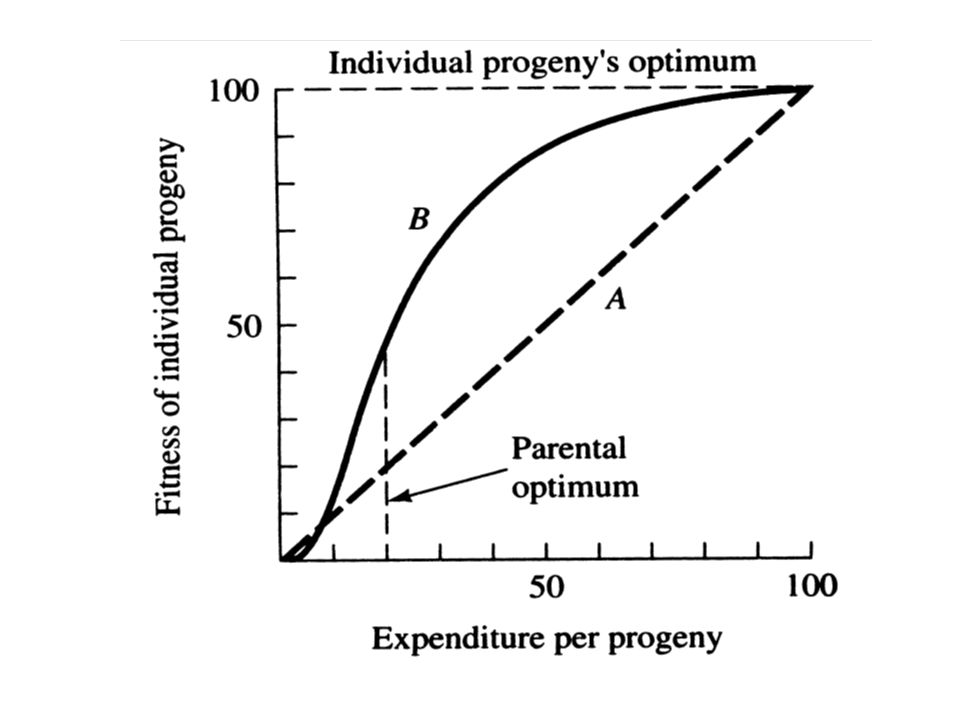
17. Trade-offs between present progeny and expectation of future offspring

18. Iteroparous organism

19. Semelparous organism

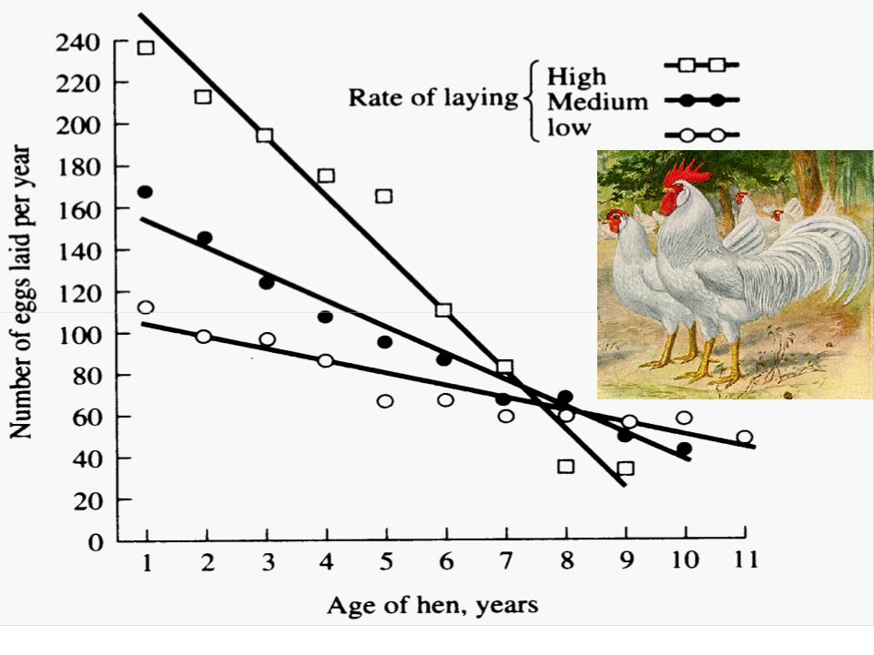
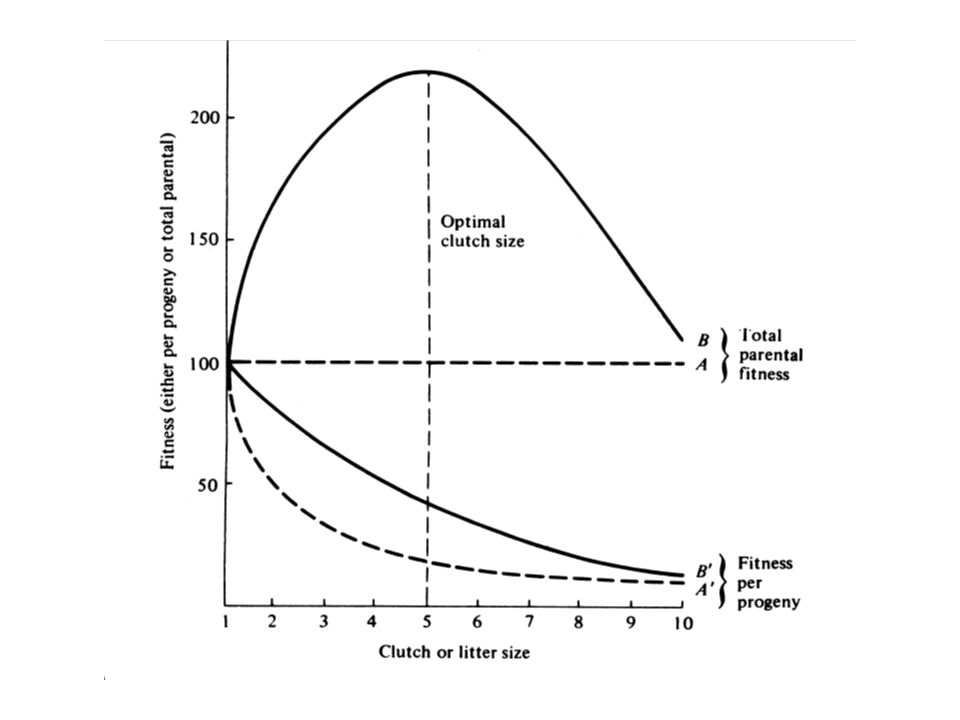
22. Patterns in Avian Clutch Sizes Altrical versus Precocial Nidicolous vs. Nidifugous Determinant vs. Indeterminant Layers Classic Experiment: Flickers usually lay 7-8 eggs, but in an egg removal experiment, a female laid 61 eggs in 63 days

23. Great Tit Parus major David Lack

24. European Starling, Sturnus vulgaris