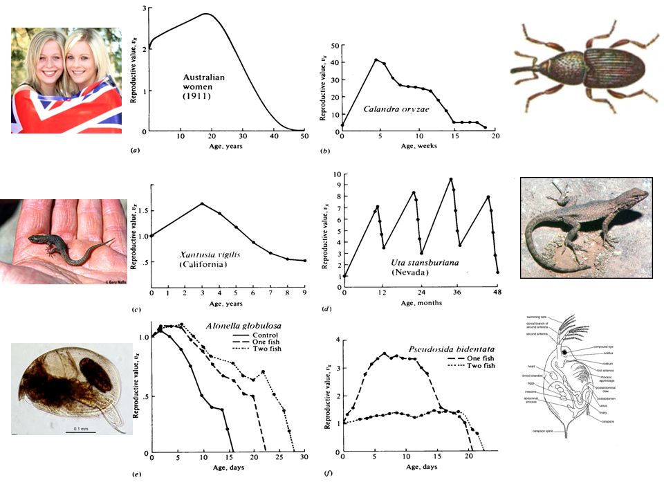
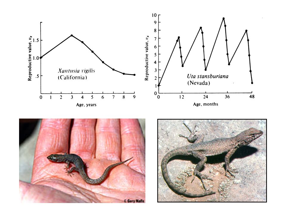
1. Life tables Age-specific probability statistics Force of mortality q x Survivorship l x l y / l x = probability of living from age x to age y Fecundity m x Realized fecundity at age x = l x m x Net reproductive rate R 0 =  l x m x Generation time T =  xl x m x Reproductive value v x =  (l t / l x ) m t E x = Expectation of further life

2. T, Generation time = average time from one gener- ation to the next (average time from egg to egg) v x = Reproductive Value = Age-specific expectation of all future offspring p.143, right hand equation “ dx ” should be “ dt ”

3. v x = m x +  (l t / l x ) m t Residual reproductive value = age-specific expectation of offspring in distant future v x * = ( l x+1 / l x ) v x+1

4. Illustration of Calculation of E x, T, R 0, and v x in a Stable Population with Discrete Age Classes _____________________________________________________________________ AgeExpectation Reproductive Weighted of Life Value Survivor-Realizedby Realized E x v x Age (x) shipFecundityFecundityFecundity l x m x l x m x x l x m x _____________________________________________________________________ 0 1.0 0.0 0.00 0.00 3.40 1.00 1 0.8 0.2 0.16 0.16 3.00 1.25 2 0.6 0.3 0.18 0.36 2.67 1.40 3 0.4 1.0 0.40 1.20 2.50 1.65 4 0.4 0.6 0.24 0.96 1.50 0.65 5 0.2 0.1 0.02 0.10 1.00 0.10 6 0.0 0.0 0.00 0.00 0.00 0.00 Sums 2.2 (GRR) 1.00 (R 0 ) 2.78 (T) _____________________________________________________________________ E 0 = (l 0 + l 1 + l 2 + l 3 + l 4 + l 5 )/l 0 = (1.0 + 0.8 + 0.6 + 0.4 + 0.4 + 0.2) / 1.0 = 3.4 / 1.0 E 1 = (l 1 + l 2 + l 3 + l 4 + l 5 )/l 1 = (0.8 + 0.6 + 0.4 + 0.4 + 0.2) / 0.8 = 2.4 / 0.8 = 3.0 E 2 = (l 2 + l 3 + l 4 + l 5 )/l 2 = (0.6 + 0.4 + 0.4 + 0.2) / 0.6 = 1.6 / 0.6 = 2.67 E 3 = (l 3 + l 4 + l 5 )/l 3 = (0.4 + 0.4 + 0.2) /0.4 = 1.0 / 0.4 = 2.5 E 4 = (l 4 + l 5 )/l 4 = (0.4 + 0.2) /0.4 = 0.6 / 0.4 = 1.5 E 5 = (l 5 ) /l 5 = 0.2 /0.2 = 1.0 v 1 = (l 1 /l 1 )m 1 +(l 2 /l 1 )m 2 +(l 3 /l 1 )m 3 +(l 4 /l 1 )m 4 +(l 5 /l 1 )m 5 = 0.2+0.225+0.50+0.3+0.025 = 1.25 v 2 = (l 2 /l 2 )m 2 + (l 3 /l 2 )m 3 + (l 4 /l 2 )m 4 + (l 5 /l 2 )m 5 = 0.30+0.67+0.40+ 0.03 = 1.40 v 3 = (l 3 /l 3 )m 3 + (l 4 /l 3 )m 4 + (l 5 /l 3 )m 5 = 1.0 + 0.6 + 0.05 = 1.65 v 4 = (l 4 /l 4 )m 4 + (l 5 /l 4 )m 5 = 0.60 + 0.05 = 0.65 v 5 = (l 5 /l 5 )m 5 = 0.1 ___________________________________________________________________________

5. Illustration of Calculation of E x, T, R 0, and v x in a Stable Population with Discrete Age Classes _____________________________________________________________________ AgeExpectation Reproductive Weighted of Life Value Survivor-Realizedby Realized E x v x Age (x) shipFecundityFecundityFecundity l x m x l x m x x l x m x _____________________________________________________________________ 0 1.0 0.0 0.00 0.00 3.40 1.00 1 0.8 0.2 0.16 0.16 3.00 1.25 2 0.6 0.3 0.18 0.36 2.67 1.40 3 0.4 1.0 0.40 1.20 2.50 1.65 4 0.4 0.6 0.24 0.96 1.50 0.65 5 0.2 0.1 0.02 0.10 1.00 0.10 6 0.0 0.0 0.00 0.00 0.00 0.00 Sums 2.2 (GRR) 1.00 (R 0 ) 2.78 (T) _____________________________________________________________________ E 0 = (l 0 + l 1 + l 2 + l 3 + l 4 + l 5 )/l 0 = (1.0 + 0.8 + 0.6 + 0.4 + 0.4 + 0.2) / 1.0 = 3.4 / 1.0 E 1 = (l 1 + l 2 + l 3 + l 4 + l 5 )/l 1 = (0.8 + 0.6 + 0.4 + 0.4 + 0.2) / 0.8 = 2.4 / 0.8 = 3.0 E 2 = (l 2 + l 3 + l 4 + l 5 )/l 2 = (0.6 + 0.4 + 0.4 + 0.2) / 0.6 = 1.6 / 0.6 = 2.67 E 3 = (l 3 + l 4 + l 5 )/l 3 = (error: extra terms) 0.4 + 0.4 + 0.2) /0.4 = 1.0 / 0.4 = 2.5 E 4 = (l 4 + l 5 )/l 4 = (error: extra terms) 0.4 + 0.2) /0.4 = 0.6 / 0.4 = 1.5 E 5 = (l 5 ) /l 5 = 0.2 /0.2 = 1.0 v 1 = (l 1 /l 1 )m 1 +(l 2 /l 1 )m 2 +(l 3 /l 1 )m 3 +(l 4 /l 1 )m 4 +(l 5 /l 1 )m 5 = 0.2+0.225+0.50+0.3+0.025 = 1.25 v 2 = (l 2 /l 2 )m 2 + (l 3 /l 2 )m 3 + (l 4 /l 2 )m 4 + (l 5 /l 2 )m 5 = 0.30+0.67+0.40+ 0.03 = 1.40 v 3 = (l 3 /l 3 )m 3 + (l 4 /l 3 )m 4 + (l 5 /l 3 )m 5 = 1.0 + 0.6 + 0.05 = 1.65 v 4 = (l 4 /l 4 )m 4 + (l 5 /l 4 )m 5 = 0.60 + 0.05 = 0.65 v 5 = (l 5 /l 5 )m 5 = 0.1 ___________________________________________________________________________

8. Stable age distribution Stationary age distribution

9. Intrinsic rate of natural increase (per capita) r = b – d when birth rate exceeds death rate (b > d), r is positive when death rate exceeds birth rate (d > b), r is negative Euler ’ s implicit equation:  e -rx l x m x = 1 (solved by iteration) If the Net Reproductive Rate R 0 is near one, r ≈ log e R 0 /T

10. J - shaped exponential population growth http://www.zo.utexas.edu/courses/THOC/exponential.growth.html

11. When R 0 equals one, r is zero When R 0 is greater than one, r is positive When R 0 is less than one, r is negative Maximal rate of natural increase, r max

12. Instantaneous rate of change of N at time t is total births (bN) minus total deaths (dN) dN/dt = bN – dN = (b – d )N = rN N t = N 0 e rt (integrated version of dN/dt = rN) log N t = log N 0 + log e rt = log N 0 + rt log R 0 = log 1 + rt (make t = T) r = log or = e r (  is the finite rate of increase)

13. Estimated Maximal Instantaneous Rates of Increase (r max, per capita per day) and Mean Generation Times ( in days) for a Variety of Organisms ___________________________________________________________________ TaxonSpecies r max Generation Time (T) ----------------------------------------------------------------------------------------------------- BacteriumEscherichia coli ca. 60.00.014 ProtozoaParamecium aurelia1.24 0.33–0.50 ProtozoaParamecium caudatum0.94 0.10–0.50 InsectTribolium confusum 0.120 ca. 80 InsectCalandra oryzae0.110(.08–.11) 58 InsectRhizopertha dominica0.085(.07–.10) ca. 100 InsectPtinus tectus0.057102 InsectGibbum psylloides0.034129 InsectTrigonogenius globulosus0.032119 InsectStethomezium squamosum0.025147 InsectMezium affine0.022183 InsectPtinus fur0.014179 InsectEurostus hilleri0.010110 InsectPtinus sexpunctatus0.006215 InsectNiptus hololeucus0.006154 MammalRattus norwegicus0.015150 MammalMicrotus aggrestis0.013171 MammalCanis domesticus0.009 ca. 1000 InsectMagicicada septendecim0.001 6050 MammalHomo “sapiens” (the sap)0.0003 ca. 7000 __________________________________________________________________ _

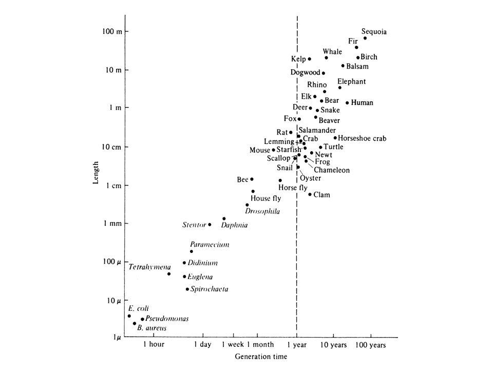
14. Inverse relationship between r max and generation time, T

16. Demographic and Environmental Stochasticity random walks, especially important in small populations Evolution of Reproductive Tactics Semelparous versus Interoparous Big Bang versus Repeated Reproduction Reproductive Effort (parental investment) Age of First Reproduction, alpha,  Age of Last Reproduction, omega, 

17. Mola mola (“Ocean Sunfish”) 200 million eggs! Poppy (Papaver rhoeas) produces only 4 seeds when stressed, but as many as 330,000 under ideal conditions

18. Indeterminant Layers

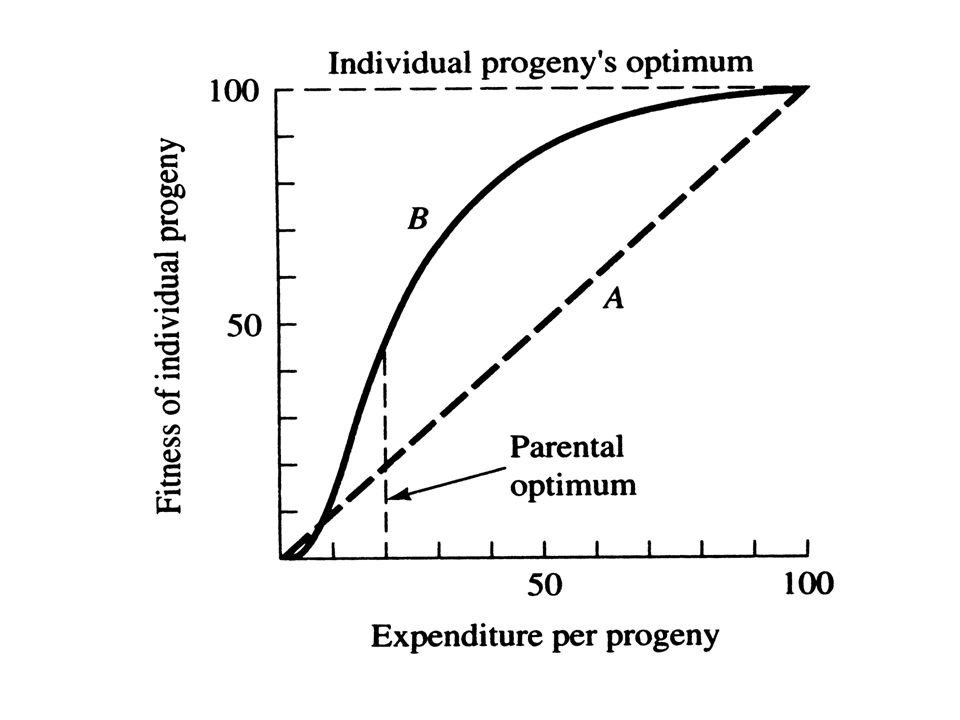
19. How much should an organism invest in any given act of reproduction? R. A. Fisher (1930) anticipated this question long ago: ‘It would be instructive to know not only by what physiological mechanism a just apportionment is made between the nutriment devoted to the gonads and that devoted to the rest of the parental organism, but also what circumstances in the life history and environment would render profitable the diversion of a greater or lesser share of available resources towards reproduction.’ [Italics added for emphasis.] Reproductive Effort Ronald A. Fisher

20. Asplanchna (Rotifer)

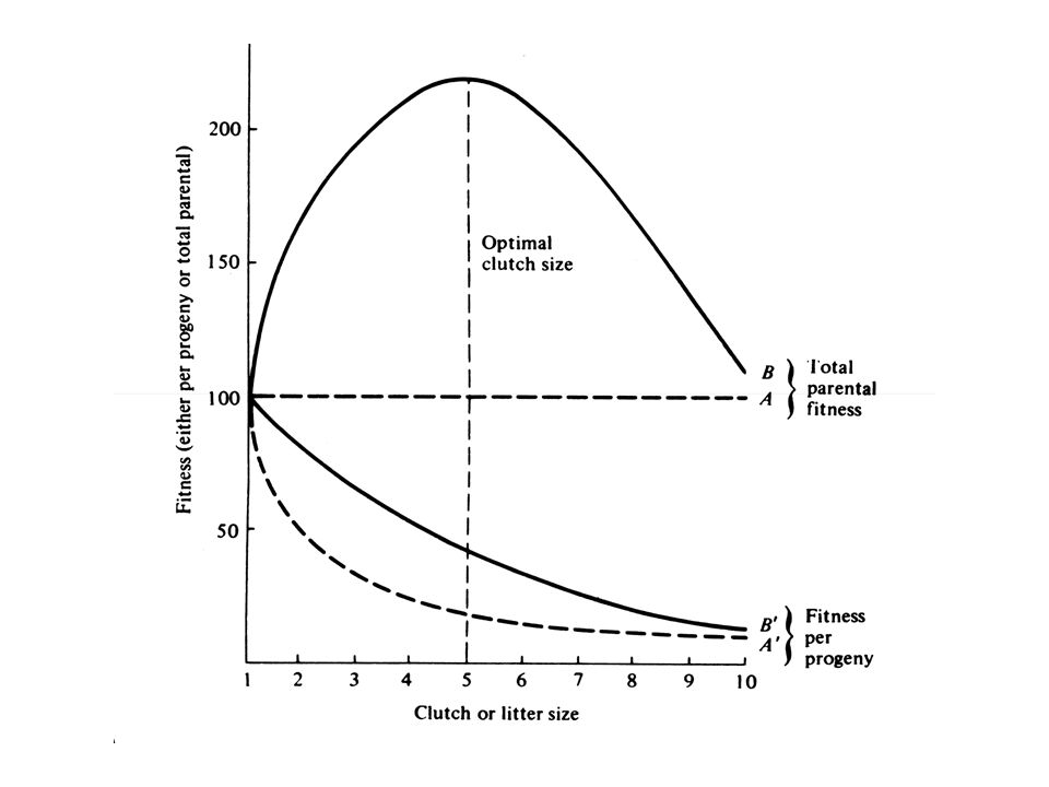
21. Trade-offs between present progeny and expectation of future offspring

22. Iteroparous organism

23. Semelparous organism

26. Patterns in Avian Clutch Sizes Altrical versus Precocial

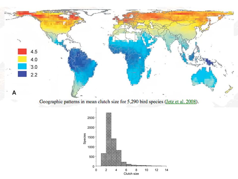
27. Patterns in Avian Clutch Sizes Altrical versus Precocial Nidicolous vs. Nidifugous Determinant vs. Indeterminant Layers N = 5290 Species

28. Patterns in Avian Clutch Sizes Open Ground Nesters Open Bush Nesters Open Tree Nesters Hole Nesters MALE (From: Martin and Ghalambor 1999)

29. Patterns in Avian Clutch Sizes Classic Experiment: Flickers usually lay 7-8 eggs, but in an egg removal experiment, a female flicker laid 61 eggs in 63 days

30. Great Tit Parus major David Lack

31. Parus major

32. European Starling, Sturnus vulgaris

33. Chimney Swift, Apus apus

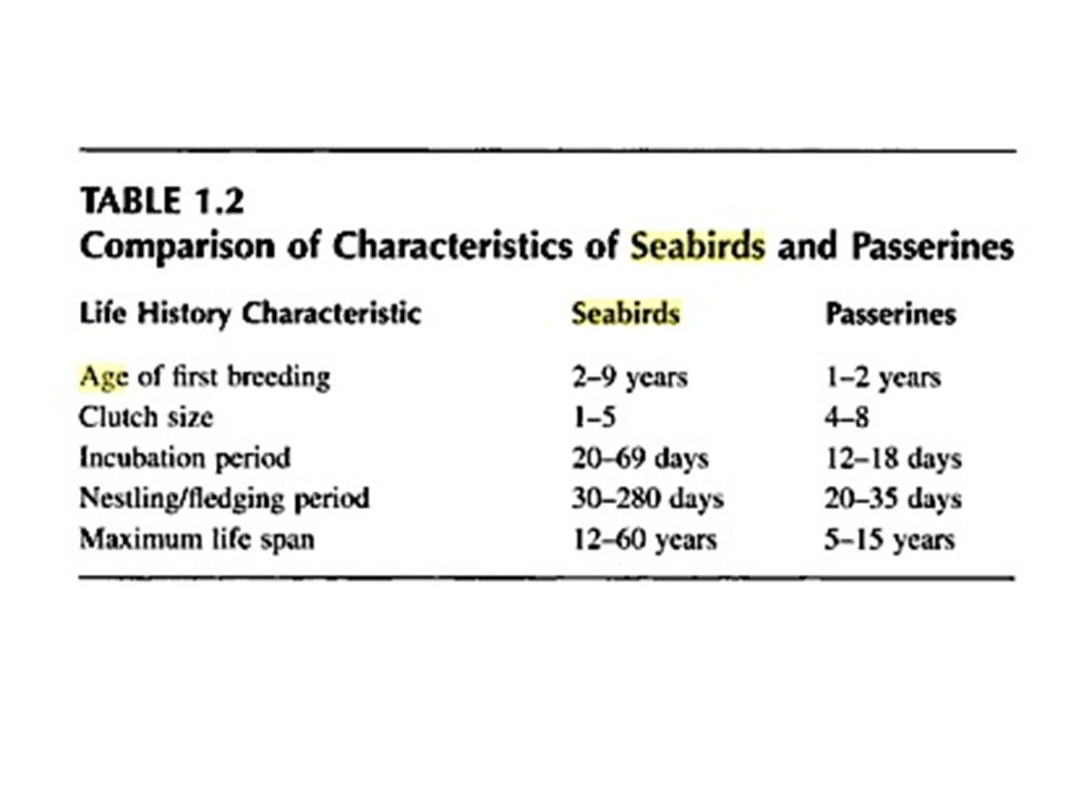
34. Seabirds (N. Philip Ashmole) Boobies, Gannets, Gulls, Petrels, Skuas, Terns, Albatrosses Delayed sexual maturity, Small clutch size, Parental care

36. Albatross Egg Addition Experiment Diomedea immutabilis An extra chick added to each of 18 nests a few days after hatching. These nests with two chicks were compared to 18 other natural “ control ” nests with only one chick. Three months later, only 5 of the 36 experimental chicks survived from the nests with 2 chicks, whereas 12 of the 18 chicks from single chick nests were still alive. Parents could not find food enough to feed two chicks and most starved to death.

37. Latitudinal Gradients in Avian Clutch Size

39. Daylength Hypothesis Prey Diversity Hypothesis Spring Bloom or Competition Hypothesis

40. Latitudinal Gradients in Avian Clutch Size Nest Predation Hypothesis Alexander Skutch ––––––>

41. Latitudinal Gradients in Avian Clutch Size Hazards of Migration Hypothesis Falco eleonora

42. Evolution of Death Rates Senescence, old age, genetic dustbin Medawar ’ s Test Tube Model p (surviving one month) = 0.9 p (surviving two months) = 0.9 2 p (surviving x months) = 0.9 x recession of time of expression of the overt effects of a detrimental allele precession of time of expression of the effects of a beneficial allele Peter Medawar

43. Age Distribution of Medawar ’ s test tubes

44. Percentages of people with lactose intolerance

45. Joint Evolution of Rates of Reproduction and Mortality Donald Tinkle Sceloporus

46. J - shaped exponential population growth http://www.zo.utexas.edu/courses/THOC/exponential.growth.html

47. Instantaneous rate of change of N at time t is total births (bN) minus total deaths (dN) dN/dt = bN – dN = (b – d )N = rN N t = N 0 e rt (integrated version of dN/dt = rN) log N t = log N 0 + log e rt = log N 0 + rt log R 0 = log 1 + rt (make t = T) r = log or = e r (  is the finite rate of increase)

48. Once, we were surrounded by wilderness and wild animals, But now, we surround them.