1. Boolean + Ranking: Querying a Database by K-Constrained Optimization Joint work with: Seung-won Hwang, Kevin C. Chang, Min Wang, Christian A. Lang, Yuan-chi Chang Presented By Rashmi Pagadala(1000574860)Swetta Bhaskar(1000568628)

2. Introduction K- Constrained Optimization Query Query Q = ( B, O, k ) B – Qualifying Constraint O – Quantifying Constraint k – number of tuples

3. Many queries naturally combine Boolean and ranking Information retrieval Ranking query: Top 5 ranked by gpa + Database applications on Web Traditional databases Boolean query: dept = CS and year = 2 Qualifying constraint Quantifying function R: gpa B: dept = CS and year = 2 Find top answers

4. Boolean + Ranking form a coherent goal function Boolean B + Ranking R = Goal function G For a tuple t G(t) = B(t)*R(t) = R(t) if B(t) is true 0 if B(t) is false (ie, lowest score)

5. Motivating scenarios Data retrieval:  Find houses in certain price range with good price/sqrft ratio Data analysis:  Find products with highest sale increase in consecutive years Select h.address from House h Where h.price ≤ 200k ν h.price ≥ 400k Order by h.size/|h.price-300k| Limit 1 Select h.address from House h, CrimeRate c Where h.price ≤ 200k ν h.price ≥ 400k and h.zipcode = c.zipcode Order by h.size/|h.price-300k| *c.crimerate -1 Limit 10 Select itemid from Sales s1, Sales s2 Where s1.itemid = s2.itemid and s2.year – s1.year = 1 Order by s2.sale – s1.sale Limit 10

6. Current techniques lack of global search mechanism If evaluated as separate operators If search by an overall goal function G as a ranking function Boolean query B ……… Ranking query R  Current techniques restrict G to be monotonic  Current techniques optimize only condition-by-condition D Boolean query B Ranking query R D RB Goal function G

7. The nature of Boolean + Ranking is K-constrained optimization query Optimize goal function G over database D h.size/|h.price-300k| [ h.price ≤ 200k ν h.price ≥ 400k ] AddrZipPriceSize 1.Oak park, Chicago 60644600K4500 2.Mattis, Champaign 61821350K2000 3.… 150K1000 4.… 250K2000 5.… 300K3500 6.… 80K500 Goal function G Database D D G

8. Our Goal: Evaluate query as its nature suggests! Optimize G over D Function optimization of G Discrete state search over D G D D OPT*

9. Query Mechanism Discrete State Search Search over a discrete set of index nodes to find the satisfying data tuples Continuous Function Optimization Optimize the goal function G over the domain of a database

10. Challenge 1: What is the search mechanism?

11. We encode as A* because it’s optimal What A* is: Finding the shortest path Why we choose: Completeness and optimality with proper heuristics  Complete: guarantee to find shortest path  Optimal: visit least number of nodes origin destination 5 2 9 6 3 5 1 1 7

12. The To do : Discrete state search perspective ( indices) Shortest path problem (Encoding)

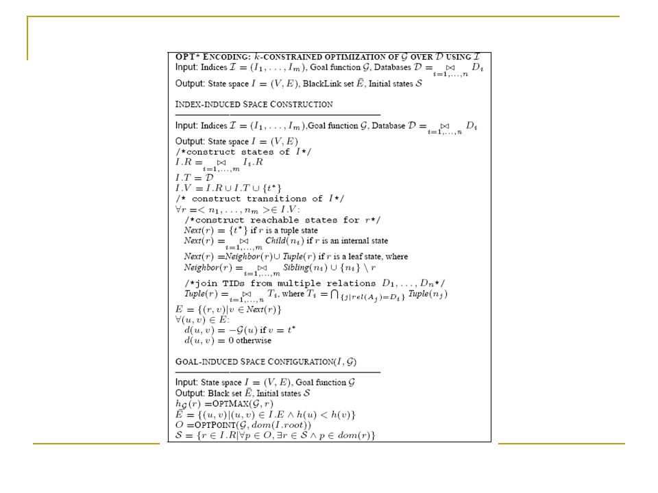
13. Index –Induced State Space: A*-Driven Construction K constrained optimization State space induced by indices: state & route I i over relation D i I i= (V,E), where V=RUT Dom(n i ),n i €R The reachable node depends on t he type of n Each node is referred to as I.V and I.E.

14. 250 3000 350 100 150040004500 600 We view compound index as discrete space 250-600 0- 250 100-2500-100350- 600 250- 350 521 ……… b1b1 b3b3 b2b2 b7b7 b6b6 3000- 4500 0- 3000 1500- 3000 0- 1500 4000- 6000 3000- 4000 51 ……… a1a1 a6a6 a3a3 a2a2 a7a7 size Price (k) 1 5 2 3 4 6

15. 250 3000 350 100 150040004500 600 We view compound index as discrete space M 11 M 22 M 32 M 23 M 33 M 66 M 77 M67M67 M 76 M 55 M 56 M 75 15 4 2 250-600 0- 250 100-2500-100350- 600 250- 350 521 ……… b1b1 b3b3 b2b2 b7b7 b6b6 3000- 4500 0- 3000 1500- 3000 0- 1500 4000- 6000 3000- 4000 51 ……… a1a1 a6a6 a3a3 a2a2 a7a7 size Price (k) 1 5 2 3 4 6 M ij =(a i, b j ) … …

16. 250 3000 350 100 150040004500 600 We view compound index as discrete space M 11 M 22 M 32 M 23 M 33 M 66 M 77 M67M67 M 76 M 55 M 56 M 75 15 4 2 250-600 0- 250 100-2500-100350- 600 250- 350 521 ……… b1b1 b3b3 b2b2 b7b7 b6b6 3000- 4500 0- 3000 1500- 3000 0- 1500 4000- 6000 3000- 4000 51 ……… a1a1 a6a6 a3a3 a2a2 a7a7 size Price (k) 1 5 2 3 4 6 M ij =(a i, b j ) conceptually, combined space …

17. Mapping the Space : state & transition States: Index graph,Composite graph Composite graph is categorized: Region U Tuples Region state: #Internal state #Leaf state Tuple state Transition: Internal state-Branch in( top down ) Leaf state-Branch out( bottom up) Cartesian product + intersection of node

18. Example Given a set of states constructed from the set of index graph I considering the transitions among the states. To reach tuple 1. The search, in principle, should follow those transitions to look for the tuple states maximizing the goal function. For instance, suppose we decide to start from the root of the graph M11. This essentially follows a top-down search strategy. The search may follow the path M11 →M33 → M77 → 1 to reach the target tuple state. Alternatively, as a bottom-up search, suppose we start fromM67, the search may follow an alternative route M67 → M77 → 1.

19. Encoding our problem into shortest path is challenging  How to encode:  a tuple  a path?  score of tuple  distance of path? K-constrained optimization Find a tuple with maximal score Shortest path Find a path with minimal distance

20. Therefore, we encode K-constrained opt. as: How to encode a tuple to a path?  Adding a virtual target t* only reachable through tuples How to encode maximal tuple with minimal path?  Quality of path depends solely on the tuple it passes by For tuple state t D(t, t*) = - G(t) For two states r, u D(r, u) = 0 M 55 M 11 M 22 M 32 M 23 M 33 M 66 M 77 M 67 M 76 M 75 M 56 1542 t* 0 0 0 0 - G(4) - G(1) 0 0 …

22. Challenge 2: How to guide the search?

23. We use function opt. to sketch the landscape of G Function optimization measures quality of states Function optimization enables:  1. How to define heuristics?  2. How to configure space?  3. Where to start the search? Return local optima O and upper bound score U

24. 1. Define admissible heuristics: Measure tightest upper bound H(region) = OPTMAX(G, region) ie, maximal value of G in the region To guarantee completeness  A* requires admissible heuristics, ie, estimate optimistically To ensure admissible heuristics  Function optimization gives tightest upper bound Analytical approaches Numeric analysis package

25. 2. Configure descending space: disconnect uphills To guarantee optimality  A* requires descending heuristics To ensure descending heuristics  Remove uphill links M 11 M 22 M 32 M 23 M 33 M 66 M 77 M 67 M 76 M 55 M 75 M 56 15 4 2 …

26. Find right start point: Start from local optima To guarantee correctness  Every tuple state must be reachable from start states  Taking only downhills requires start with high points To ensure reachability  Initial states should contain all local optima M 11 M 22 M 32 M 23 M 33 M 66 M 77 M 67 M 76 M 55 M 75 M 56 15 4 2 …

27. OPT SEARCH ALGORITHM

28. Putting together: Executing OPT* on the configured space M 11 M 22 M 32 M 23 M 33 M 66 M 77 M 67 M 76 M 55 M 75 M 56 15 4 2 M 57 … Search is implemented as priority queue driven traversal top-down

29. Putting together: Executing OPT* on the configured space Bottom-up approach is always better than top- down M 11 M 22 M 32 M 23 M 33 M 66 M 77 M 67 M 76 M 55 M 75 M 56 15 4 2 M 57 M 11 M 22 M 32 M 23 M 33 M 66 M 77 M 67 M 76 M 55 M 75 M 56 15 4 2 M 57 … … top-down bottom-up

30. Experiments Comparison vs.  Boolean then ranking  Ranking then boolean Metrics: node accessed = N l + N t Settings:  Benchmark queries over real dataset  Controlled queries over synthetic dataset

31. Benchmark queries Datasets:  19,706 real estate listing crawled online Queries  Q1: size * bedrms/| price-450k| : [40k<=price<=50k]  Q2: size * e bedrms / |price-350k| : [price 4000]  Q3: size/price : [bedrms=3 ν bedrms=4] BR_unclustered BR_clustered OPT* Q1Q2Q3

32. Controlled queries Datasets  Three randomly generated datasets of 100k points Uniform, gaussian, logvariatenormal Queries  Linear average queries: (eg, 0.4*a + 0.6*b)  Nearest neighbor queries: (eg, (x-3)^2 + (y-4)^2)  Join queries: (0.4*R.a + 0.6*S.b: R.c=R.d)

33. Conclusion Problem  Study K-constrained optimization queries as boolean + ranking Abstraction  Encode K-constrained optimization into shortest path problem Framework  Develop OPT* to process K-constrained optimization

34. References: Boolean + Ranking: Querying a Database by K-Constrained Optimization Joint work with: Seung-won Hwang, Kevin C. Chang, Min Wang, Christian A. Lang, Yuan-chi Chang W. H. Press, S. A. Teukolsky, W. T.Vetterling, and B. P.Flannery. CAMBRIDGE UNIVERSITY PRESS, 2 nd Edition, 1992. www-forward.cs.uiuc.edu/talks/2006/asopt-sigmod06-zzhang-jun06 http://portal.acm.org/citation.cfm?id=1142473.1142515

35. THANK YOU ! Questions?