Download presentation
Presentation is loading. Please wait.

1
6. Maxwell’s Equations In Time-Varying Fields
7e Applied EM by Ulaby and Ravaioli

2
Chapter 6 Overview

3
Maxwell’s Equations In this chapter, we will examine Faraday’s and Ampère’s laws

4
Faraday’s Law Electromotive force (voltage) induced by time-varying magnetic flux:
 induced by time-varying magnetic flux:")
5
Three types of EMF

6
Stationary Loop in Time-Varying B

7
cont.

8
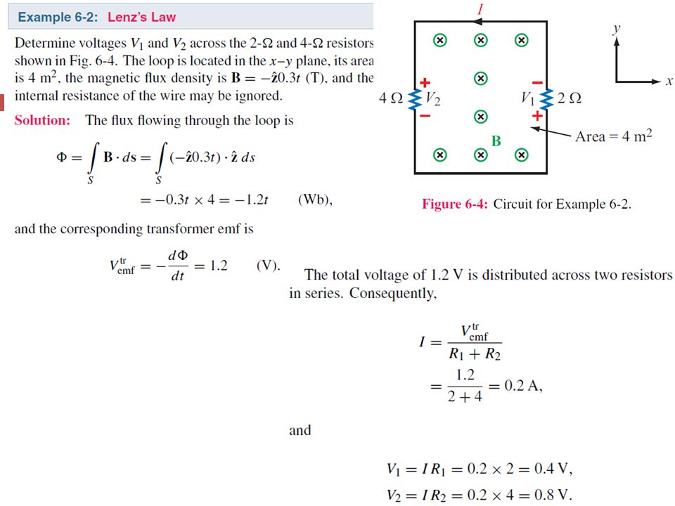
Example 6-1 Solution

11
Ideal Transformer

12
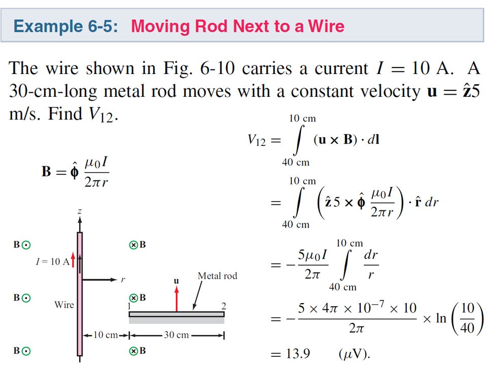
Motional EMF Magnetic force on charge q moving with velocity u in a magnetic field B: This magnetic force is equivalent to the electrical force that would be exerted on the particle by the electric field Em given by This, in turn, induces a voltage difference between ends 1 and 2, with end 2 being at the higher potential. The induced voltage is called a motional emf

13
Motional EMF

14
Example 6-3: Sliding Bar Note that B increases with x
The length of the loop is related to u by x0 = ut. Hence

16
EM Motor/ Generator Reciprocity
Motor: Electrical to mechanical energy conversion Generator: Mechanical to electrical energy conversion

17
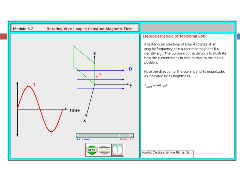
EM Generator EMF As the loop rotates with an angular velocity ω about its own axis, segment 1–2 moves with velocity u given by Also: Segment 3-4 moves with velocity –u. Hence:

19
Tech Brief 12: EMF Sensors
Piezoelectric crystals generate a voltage across them proportional to the compression or tensile (stretching) force applied across them. Piezoelectric transducers are used in medical ultrasound, microphones, loudspeakers, accelerometers, etc. Piezoelectric crystals are bidirectional: pressure generates emf, and conversely, emf generates pressure (through shape distortion).
 force applied across them. Piezoelectric transducers are used in medical ultrasound, microphones, loudspeakers, accelerometers, etc. Piezoelectric crystals are bidirectional: pressure generates emf, and conversely, emf generates pressure (through shape distortion).")
20
Faraday Accelerometer
The acceleration a is determined by differentiating the velocity u with respect to time

21
The Thermocouple The thermocouple measures the unknown temperature T2 at a junction connecting two metals with different thermal conductivities, relative to a reference temperature T1. In today’s temperature sensor designs, an artificial cold junction is used instead. The artificial junction is an electric circuit that generates a voltage equal to that expected from a reference junction at temperature T1.

22
Displacement Current This term must represent a current
This term is conduction current IC Application of Stokes’s theorem gives: Cont.

23
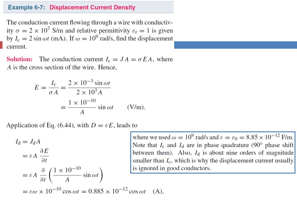
Displacement Current Define the displacement current as:
The displacement current does not involve real charges; it is an equivalent current that depends on

24
Capacitor Circuit I2 = I2c + I2d I2c = 0 (perfect dielectric)
Given: Wires are perfect conductors and capacitor insulator material is perfect dielectric. For Surface S2: I2 = I2c + I2d I2c = 0 (perfect dielectric) For Surface S1: I1 = I1c + I1d (D = 0 in perfect conductor) Conclusion: I1 = I2
 For Surface S1: I1 = I1c + I1d. (D = 0 in perfect conductor) Conclusion: I1 = I2.")
26
Boundary Conditions

27
Charge Current Continuity Equation
Current I out of a volume is equal to rate of decrease of charge Q contained in that volume: Used Divergence Theorem

28
Charge Dissipation Question 1: What happens if you place a certain amount of free charge inside of a material? Answer: The charge will move to the surface of the material, thereby returning its interior to a neutral state. Question 2: How fast will this happen? Answer: It depends on the material; in a good conductor, the charge dissipates in less than a femtosecond, whereas in a good dielectric, the process may take several hours. Derivation of charge density equation: Cont.

29
Solution of Charge Dissipation Equation
For copper: For mica: = 15 hours

30
EM Potentials Static condition Dynamic condition
Dynamic condition with propagation delay: Similarly, for the magnetic vector potential:

31
Time Harmonic Potentials
If charges and currents vary sinusoidally with time: Also: we can use phasor notation: Maxwell’s equations become: with Expressions for potentials become:

32
Cont.

33
Cont.

34
Example 6-8 cont. Cont.

35
Example 6-8 cont.

36
Summary

Similar presentations


 The magnetic.>")
 i.>")


 Lenz’s Law (direction of induced.>")


