1. Self Organizing Maps: Clustering With unsupervised learning there is no instruction and the network is left to cluster patterns. All of the patterns within a cluster will be judged as being similar. Cluster algorithms form groups referred to as clusters and the arrangement of clusters should reflect two properties: –Patterns within a cluster should be similar in some way. –Clusters that are similar in some way should be close together.

2. The Self-organizing Feature Map The input units correspond in number to the dimension of the training vectors. The output units act as prototypes. This network has three inputs and five cluster units. Each unit in the input layer is connected to every unit in the cluster layer.

3. How does a cluster unit act as a prototype? w 2,1 w 1,1 x1x1 x2x2 p1p1 x 2 coordinatex 1 coordinate w 1,1 w 2,1 The input layer takes coordinates from the input space. The weights adapt during training, and when learning is complete each cluster unit will have a position in the input space determined by weights.

4. Radius 1 Radius 2 Winning unit, only one to update if radius=0 Units to be updated when radius=1 Units to be updated when radius=2 The topology determines which units fall within a radius of the winning unit. The winning unit will adapt its weights in a way that moves that cluster unit even closer to the training vector. Weight updates within a radius

5. Algorithm initialize weights to random values. while not HALT for each input vector for each cluster unit calculate the distance from the training vector find unit j with the minimum distance update all weight vectors for units within the radius according to check to see if the learning rate or radius needs updating check HALT.

6. Self-Organizing Maps –On each training input, all output nodes that are within a topological distance, d T, of D from the winner node will have their incoming weights modified. d T (y i,y j ) = # nodes that must be traversed in the output layer in moving between output nodes y i and y j. –D is typically decreased as training proceeds. Fully Interconnected Input Output Partially Intraconnected

7. Example An SOFM has a 10x10 two-dimensional grid layout and the radius is initially set to 6. Find how many units will be updated after 1000 epochs if the winning unit is located in the extreme bottom right-hand corner of the grid and the radius is updated according to r = r-1 if current_epoch mod 200 = 0 Assume that epoch numbering starts at 1.

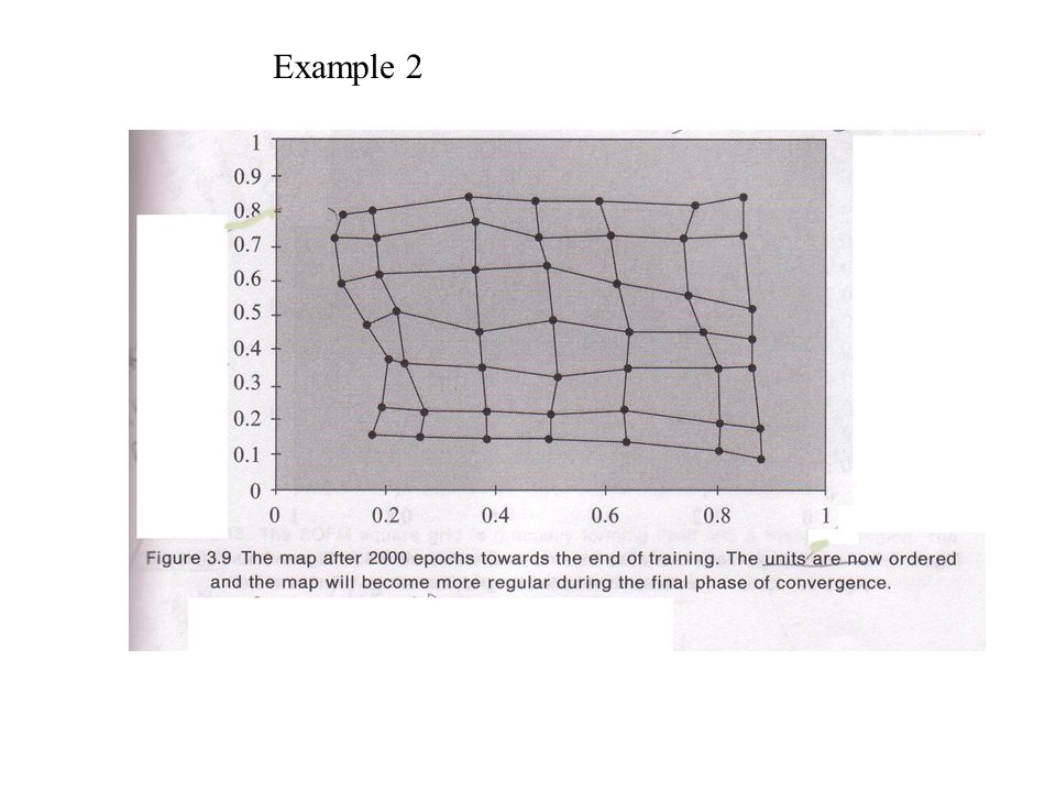
8. Example 2

11. Example 3

12. Figure 3.16 The weight vector positions converted to (x,y) coordinates after 5000 cycles through all the training data.

13. Example 3 Figure 3.18 The weight vector positions converted to (x,y) coordinates after 20000 cycles through all the training data. Figure 3.17 The weight vector positions converted to (x,y) coordinates after 10000 cycles through all the training data.

14. There Goes The Neighborhood D = 1 D = 2 D = 3 As the training period progresses, gradually decrease D. Over time, islands form in which the center represents the centroid C of a set of input vectors, S, while nearby neighbors represent slight variations on C and more distant neighbors are major variations. These neighbors may only win on a few (or no) input vectors, while the island center will win on many of the elements of S.

15. Self Organization In the beginning, the Euclidian distance d E (y l,y k ) and Topological distance d T (y l,y k ) between output nodes y l and y k will not be related. But during the course of training, they will become positively correlated: Neighbor nodes in the topology will have similar weight vectors, and topologically distant nodes will have very different weight vectors. Euclidean Neighbor Emergent Structure of Output Layer BeforeAfter Topological Neighbor

16. Example 4 An SOFM network with three inputs and two cluster units is to be trained using the four training vectors: [0.8 0.7 0.4], [0.6 0.9 0.9], [0.3 0.4 0.1], [0.1 0.1 02] and initial weights The initial radius is 0 and the learning rate is 0.5. Calculate the weight changes during the first cycle through the data, taking the training vectors in the given order. weights to the first cluster unit

17. Solution The euclidian distance of the input vector 1 to cluster unit 1 is: The euclidian distance of the input vector 1 to cluster unit 2 is: Input vector 1 is closest to cluster unit 1 so update weights to cluster unit 1:

18. Solution The euclidian distance of the input vector 2 to cluster unit 1 is: The euclidian distance of the input vector 2 to cluster unit 2 is: Input vector 2 is closest to cluster unit 1 so update weights to cluster unit 1 again: Repeat the same update procedure for input vector 3 and 4 also.

19. The angle between vectors as the measure of similarity The dot product which is sometimes called the inner product or scalar product, of two vectors v and w is given as follows: p1p1 p2p2 a The angle between non-zero vectors v and w is:

20. Weight update for dot product as measure of similarity The winning prototype index for an input vector x: index(x)=max p j.x for all j The weight updates are given by:

21. Self-Organized Maps for Robot Navigation Owen & Nehmzow (1998) Task: Autonomous robot navigation in a laboratory Goals: 1. Find a useful internal representation (i.e. map) that supports an intelligent choice of actions for the given sensory inputs 2. Let the robot build/learn the map itself - Saves the user from specifying it. - Allows the robot to handle new environments. - By learning the map in a noisy, real-world situation, the robot will be more apt to handle other noisy environments. Approach: Use an SOM to organize situation-action vectors. The emerging structure of the SOM then constitutes the robot’s functional internal representation of both the outside world and the appropriate actions to take in different regions of that world.

22. The Training Phase R 1. Record Sensory Info “Turn Right & Slow Down 2. Get correct actions 3. Input Vector = Sensory Inputs & Actions Input Output 4. Run SOM on Input Vector 5. Update Winner & Neighbors

23. The Testing Phase R 1. Record Sensory Info 2. Input Vector = Sensory Inputs & No Actions Input Output 3. Run SOM on Input Vector 4. Read Recommended Actions from the Winner’s Weight Vector A

24. Clustering of Perceptual Signatures The general closeness of successive winners shows a correlation between points & distances in the objective world and the robot’s functional view of that world. Note: A trace of the robot’s path on a map of the real world (i.e. lab floor) would have ONLY short moves. The sequence of winner nodes during the testing phase of a typical navigation task.

25. SOM for Navigation Summary SOM Regions = Perceptual Landmarks = Sets of similar perceptual patterns Navigation = Association of actions with perceptual landmarks Behavior is controlled by the robot’s subjective functional interpretation of the world, which may abstract the world into a few key perceptual categories. No extensive objective map of the entire environment is required. Useful maps are user & task centered. Robustness (Fault Tolerance): The robot also navigates successfully when a few of its sensors are damaged => The SOM has generalized from the specific training instances. Similar neuronal organizations, with correlations between points in the visual field and neurons in a brain region, are found in many animals.

26. Brain Maps

27. Topological Neural Networks Bear, Connors & Paradiso (2001). Neuroscience: Exploring The Brain. Pg. 474.

28. Tonotopic Maps in the Auditory System Spiral Ganglion Ventral Cochlear Nucleus Superior Olive Inferior Colliculus MGN Auditory Cortex Cochlea (Inner Ear) 20 kHz 4 kHz 1 kHz 10 kHz Cochlea Sp. Gang. Cochlear Nucleus Source Localization Via Delay Lines 20 kHz4 kHz1 kHz10 kHz Tonotopy preserved through all 7 levels of processing

29. Brain Facts, pg. 14, NeuroScience Society

30. Source Localization using Delay Lines Source Location Detection Neurons: Need 2 simultaneous inputs to fire Transformer Neurons: Convert sound frequency into a neural firing pattern, which is phase-locked to the sound waves (although lower freq). Right Ear Left Ear Left 90 o Left 45 o Right 90 o Right 45 o Straight Ahead! Owls have different ear heights, so they can use the same mechanism for horizontal and vertical localization Topological Map = Similar dirs detected by neighboring cells.

31. Occular Dominance & Orientation Columns Right eyeLeft eyeRight eyeLeft eye Layers 5 & 6 of V1 Neural Response (Firing rate) 0o0o 90 o -90 o 2 Topological Maps Cells respond to lines at particular angles, and nearby cells respond to similar angles. Regions of cells respond to the same eye. Retina LGN Orientation Angle