1. 12 Nonlinear Mechanics and Chaos Dr. Jen-Hao Yeh Prof. Anlage

2. This is a brief introduction to the ideas and concepts of nonlinear mechanics, and a discussion of various quantitative methods for analyzing such problems We will focus on the driven damped pendulum (DDP)

3. LinearNonlinear easyhard specialgeneral analyticalnumerical Superposition principle Chaos

4. Linear Nonlinear Chaotic

5. Driven, Damped Pendulum (DDP) We expect something interesting to happen as  → 1, i.e. the driving force becomes comparable to the weight

6. A Route to Chaos

7. NDSolve in Mathematica

8. Driven, Damped Pendulum (DDP) Period = 2  = 1 For all following plots:

9. Small Oscillations of the Driven, Damped Pendulum  << 1 will give small oscillations  (t) t  = 0.2 After the initial transient dies out, the solution looks like Periodic “attractor” Linear

10. Small Oscillations of the Driven, Damped Pendulum  << 1 will give small oscillations 1)The motion approaches a unique periodic attractor independent of initial conditions 2)The motion is sinusoidal with the same frequency as the drive

11. Moderate Oscillations of the Driven, Damped Pendulum  < 1 and the nonlinearity becomes significant… This solution gives from the  3 term: Try Since there is no cos(3  t) on the RHS, it must be that all develop a cos(3  t) time dependence. Hence we expect: We expect to see a third harmonic as the driving force grows

12. Harmonics

13.  = 0.9  (t) t t cos(  t) -cos(3  t) Moderate Driving: The Nonlinearity Distorts the cos(  t) The third harmonic distorts the simple The motion is periodic, but …

14. Even Stronger Driving: Complicated Transients – then Periodic!  = 1.06  (t) t After a wild initial transient, the motion becomes periodic After careful analysis of the long-term motion, it is found to be periodic with the same period as the driving force

15. Slightly Stronger Driving: Period Doubling  = 1.073  (t) t After a wilder initial transient, the motion becomes periodic, but period 2! The long-term motion is TWICE the period of the driving force! A SUB-Harmonic has appeared

16. Harmonics and Subharmonics Subharmonic

17. Slightly Stronger Driving: Period 3  (t) t  = 1.077 Period 3 The period-2 behavior still has a strong period-1 component Increase the driving force slightly and we have a very strong period-3 component

18. Multiple Attractors For the drive damped pendulum: Different initial conditions result in different long-term behavior (attractors)  (t) t  = 1.077 The linear oscillator has a single attractor for a given set of initial conditions Period 3 Period 2

19. Period Doubling Cascade  = 1.06  = 1.078  = 1.081  = 1.0826 Period 1 Period 2 Period 4 Period 8 Early-time motion Close-up of steady-state motion  (t) t t

20. Period Doubling Cascade  = 1.06  = 1.078  = 1.081  = 1.0826

21. n period  n interval (  n+1 -  n ) 1 1 → 2  0.0130 2 2 → 4  0.0028 3 4 → 8  0.0006 4 8 → 16  ‘Bifurcation Points’ in the Period Doubling Cascade Driven Damped Pendulum The spacing between consecutive bifurcation points grows smaller at a steady rate:  = 4.6692016 is called the Feigenbaum number ‘≈’ → ‘=’ as n → ∞ The limiting value as n → ∞ is  c = 1.0829. Beyond that is … chaos!

22. Period Doubling Cascade Period doubling continues in a sequence of ever-closer values of  Such period-doubling cascades are seen in many nonlinear systems Their form is essentially the same in all systems – it is “universal”

23. Period infinity

24.  (t) t  = 1.105 Chaos! The pendulum is “trying” to oscillate at the driving frequency, but the motion remains erratic for all time

25. Chaos Nonperiodic Sensitivity to initial conditions

26. Sensitivity of the Motion to Initial Conditions Start the motion of two identical pendulums with slightly different initial conditions Does their motion converge to the same attractor? Does it diverge quickly? Two pendulumsare given different initial conditions Follow their evolution and calculate For a linear oscillator Long-term attractor Transient behavior The initial conditions affect the transient behavior, the long-term attractor is the same Hence Thus the trajectories will converge after the transients die out

27. Convergence of Trajectories in Linear Motion Take the logarithm of |  (t)| to magnify small differences. Plotting log 10 [|  (t)|] vs. t should be a straight line of slope –  plus some wiggles from the ln[|cos(  1 t –  1 )|] term Note that log 10 [x] = log 10 [e] ln[x]

28. Log 10 [|  (t)|] t  = 0.1  (0) = 0.1 Radians Convergence of Trajectories in Linear Motion The trajectories converge quickly for the small driving force (~ linear) case This shows that the linear oscillator is essentially insensitive to its initial conditions!

29. Log 10 [|  (t)|] t  = 1.07  (0) = 0.1 Radians Convergence of Trajectories in Period-2 Motion The trajectories converge more slowly, but still converge

30. Log 10 [|  (t)|] t  = 1.105  (0) = 0.0001 Radians Divergence of Trajectories in Chaotic Motion The trajectories diverge, even when very close initially  (16) ~ , so there is essentially complete loss of correlation between the pendulums If the motion remains bounded, as it does in this case, then  can never exceed 2 . Hence this plot will saturate Extreme Sensitivity to Initial Conditions Practically impossible to predict the motion

31. The Lyapunov Exponent = Lyapunov exponent < 0: periodic motion in the long term > 0: chaotic motion

32. LinearNonlinear Chaos Drive period Harmonics, Subharmonics, Period-doubling Nonperiodic, Extreme sensitivity < 0 > 0

33. t  = 1.13  (0) = 0.001 Radians What Happens if we Increase the Driving Force Further? Does the chaos become more intense?  (t) t Log 10 [|  (t)|] Period 3 motion re-appears! With increasing  the motion alternates between chaotic and periodic

34. t  = 1.503  (0) = 0.001 Radians What Happens if we Increase the Driving Force Further? Does the chaos re-appear?  (t) Log 10 [|  (t)|] Chaotic motion re-appears! t This is a kind of ‘rolling’ chaotic motion

35.  = 1.503  (t) t  (0) = 0.001 Radians Divergence of Two Nearby Initial Conditions for Rolling Chaotic Motion Chaotic motion is always associated with extreme sensitivity to initial conditions Periodic and chaotic motion occur in narrow intervals of 

36. Bifurcation Diagram

37. Period Doubling Cascade Period doubling continues in a sequence of ever-closer values of  Such period-doubling cascades are seen in many nonlinear systems Their form is essentially the same in all systems – it is “universal” Sub-harmonic frequency spectrum Driven Diode experiment F 0 cos(  t)  /2

38. Period Doubling Cascade Period doubling continues in a sequence of ever-closer values of  Such period-doubling cascades are seen in many nonlinear systems Their form is essentially the same in all systems – it is “universal” The Brain-behaviour Continuum: The Subtle Transition Between Sanity and Insanity By Jose Luis. Perez Velazquez Fig. 12.9, Taylor A period doubling cascade in convection of mercury in a small convection cell. The plots show the temperature at one fixed point in the cell as a function of time, for four successively larger temperature gradients as given by the parameter R/R c

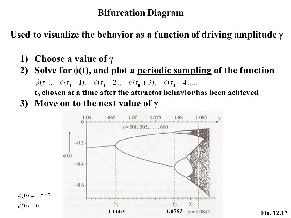
39. Bifurcation Diagram Used to visualize the behavior as a function of driving amplitude  1)Choose a value of  2)Solve for  (t), and plot a periodic sampling of the function t 0 chosen at a time after the attractor behavior has been achieved 3)Move on to the next value of  Fig. 12.17 1.0663 1.0793

40. Period 1 Period 2 Period 4 Period 8  (t) t  = 1.06  = 1.078  = 1.081  = 1.0826 Construction of the Bifurcation Diagram Period 6 window

41.  = 1.503  (t) t  (0) = 0.001 Radians The Rolling Motion Renders the Bifurcation Diagram Useless As an alternative, plot

42. Previous diagram range Mostly chaos Period-3 Mostly chaos Period-1 followed by period doubling bifurcation Mostly chaos Bifurcation Diagram Over a Broad Range of  Rolling Motion (next slide)

43. Period-1 Rolling Motion at  = 1.4  = 1.4 t t Even though the pendulum is “rolling”, is periodic  (t)

44. An Alternative View: State Space Trajectory Plot vs. with time as a parameter Fig. 12.20, 12.21  (t) t  = 0.6 First 20 cycles Cycles 5 -20 start periodic attractor

45. An Alternative View: State Space Trajectory Plot vs. with time as a parameter Fig. 12.22  = 0.6 First 20 cycles Cycles 5 -20 start The state space point moves clockwise on the orbit The periodic attractor: [, ] is an ellipse periodic attractor

46. State Space Trajectory for Period Doubling Cascade  = 1.078  = 1.081 Period-2Period-4 Plotting cycles 20 to 60 Fig. 12.23

47. State Space Trajectory for Chaos  = 1.105 Cycles 14 - 21 Cycles 14 - 94 The orbit has not repeated itself…

48. State Space Trajectory for Chaos  = 1.5  =  0 /8 Cycles 10 – 200 Chaotic rolling motion Mapped into the interval –  <  <  This plot is still quite messy. There’s got to be a better way to visualize the motion …

49. The Poincaré Section Similar to the bifurcation diagram, look at a sub-set of the data 1)Solve for  (t), and construct the state-space orbit 2)Plot a periodic sampling of the orbit with t 0 chosen after the attractor behavior has been achieved  = 1.5  =  0 /8 Samples 10 – 60,000 Enlarged on the next slide

50. The Poincaré Section is a Fractal The Poincaré section is a much more elegant way to represent chaotic motion

51. The Superconducting Josephson Junction as a Driven Damped Pendulum     = phase difference of SC wave-function across the junction I 1 2 (Tunnel barrier) The Josephson Equations

52. Radio Frequency (RF) Superconducting Quantum Interference Devices (SQUIDs) L L JJ RC  Flux Quantization in the loop I(t) IcIc

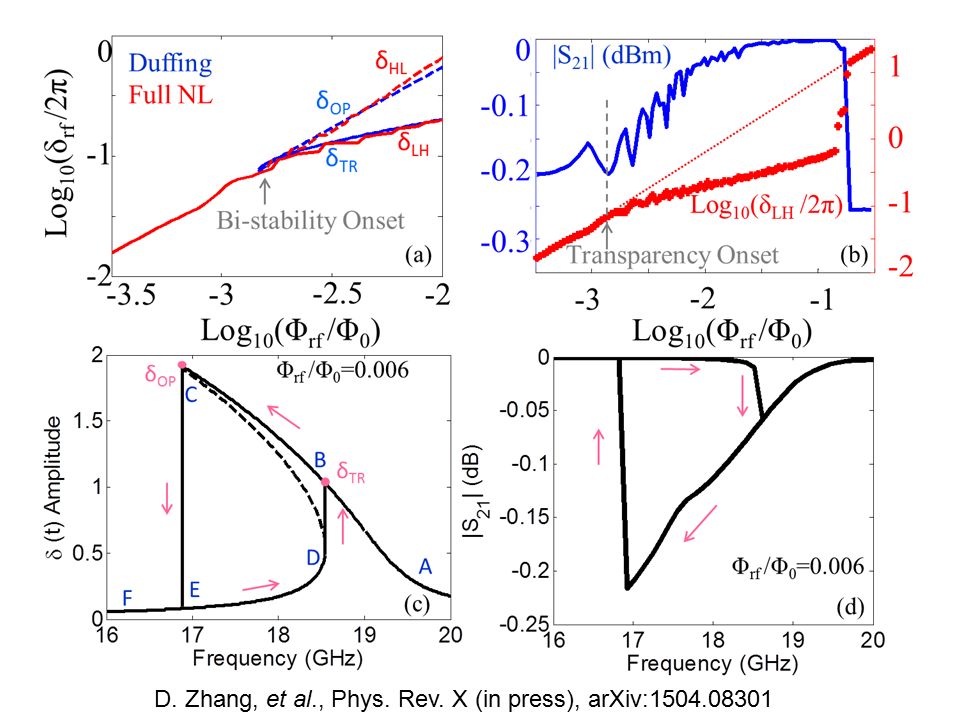
53. Single rf-SQUIDD. Zhang, et al., Phys. Rev. X (in press), arXiv:1504.08301

55. THz Emission from the Intrinsic Josephson Effect A classic problem in nonlinear physics DC voltage on junction creates an oscillating  (t), which in turn creates an AC current that radiates  0 = h/2e = 2.07 x 10 -15 Tm 2 Best emission is seen when the crystal is partially heated above T c ! Results are extremely sensitive to details (number of layers, edge properties, type of material, width of mesa, etc.) Many competing states do not show emission Emission enhanced near cavity mode resonances → requires non-uniform current injection, assisted by inhom. heating,  -phase kinks, crystal defects L. Ozyuzer, et al., Science 318, 1291 (2007)

56. Linear Maps for “Integrable” systems !! Non-Linear Maps for “Chaotic” systems !! 0 The “Chaos” arises due to the shape of the boundaries enclosing the system. Chaos in Newtonian Billiards Imagine a point-particle trapped in a 2D enclosure and making elastic collisions with the walls Describe the successive wall-collisions with a “mapping function” Computer animation of extreme sensitivity to initial conditions for the stadium billiardanimation