1. Steady-state tracking & sys. types G(s) C(s) + - r(s) e y(s) plant controller

2. G1(s) + - r(s) e G2(s) d(s) A B y(s)

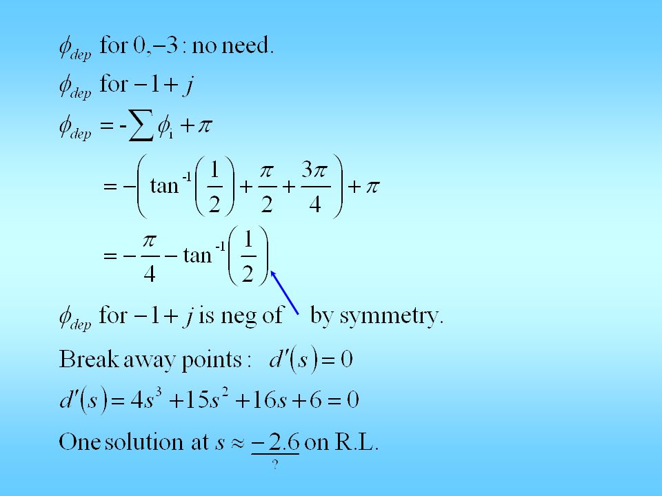
3. The root locus technique 1.Obtain closed-loop TF and char eq d(s) = 0 2.Re-arrange to get 3.Mark zeros with “o” and poles with “x” 4.High light segments of x-axis and put arrows 5.Decide #asymptotes, their angles, and x-axis meeting place: 6.Determine jw-axis crossing using Routh table 7.Compute breakaway: 8.Departure/arrival angle:

4. rlocus([1 3], conv([1 2 2 0],[1 11 30]))

5. Example: motor control The closed-loop T.F. from θ r to θ is:

6. What is the open-loop T.F.? The o.l. T.F. of the system is: But for root locus, it depends on which parameter we are varying. 1.If K P varies, K D fixed, from char. poly.

7. The o.l. T.F. for K P -root-locus is the system o.l. T.F. In general, this is the case whenever the parameter is multiplicative in the forward loop. 2.If K D is parameter, K P is fixed From

8. What if neither is fixed? Multi-parameter root locus? –Some books do this Additional specs to satisfy? –Yes, typically –Then use this to reduce freedom The o.l. T.F. of the system is: It is type 1, tracks step with 0 error Suppose ess to ramp must be <=1

9. Since ess to ramp = 1/Kv Kv = lim_s->0 {sGol(s)} =2KP/(4+2KD) Thus, ess=(4+2KD)/2KP Design to just barely meet specs: ess=1 (4+2KD)/2KP = 1 4+2KD=2KP

10. >> rlocus([2 2], [1 10 0 0]); >> grid; >> axis equal;

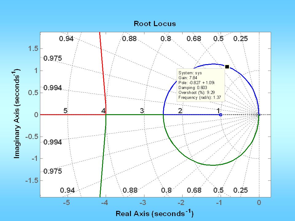
11. The grid line rays correspond to  The semi circles corresponds to  n If there is a design specification: Mp <= 10 %, then we need  >= 0.6 Select data point tool, and click at a point on the root locus with  >= 0.6

13. Desired K P = 7.84 Closed loop dominant pole at -0.827+-1.09i Pole damping ratio is 0.603 Undamped frequency is 1.37 Estimated overshoot is 9.29%

14. With KP = 7.84 Design specs for ess=1 required 4+2KD=2KP KD=KP-2 = 5.84 >> roots([1 10 15.68 15.68]) ans = -8.3464 + 0.0000i -0.8268 + 1.0932i -0.8268 - 1.0932i

15. Closed loop TF is: >>max(y) ans = 1.0915 Actual Mp=9.15%

16. More examples 1. No finite zeros, o.l. poles: 0,-1,-2 Real axis: are on R.L. Asymp: #: 3

17. -axis crossing: char. poly:

18. >> rlocus(1,[1 3 2 0]) >> grid >> axis equal

19. Example: Real axis: (-2,0) seg. is on R.L.

20. For

21. Break away point:

22. -axis crossing: char. poly:

23. >> rlocus(1, conv([1 2 0], [1 2 2])) >> axis equal >> sgrid

24. Example: in prev. ex., change s+2 to s+3

26. -axis crossing: char. poly:

27. >> rlocus(1, conv([1 3 0], [1 2 2])) >> axis equal >> sgrid