1. École Doctorale des Sciences de l'Environnement d’Île-de-France Année Universitaire 2014-2015 Modélisation Numérique de l’Écoulement Atmosphérique et Assimilation de Données Olivier Talagrand Cours 4 23 Avril 2015

2. After N. Gustafsson

3. Optimal Interpolation Random field  (  ) Observation network  1,  2, …,  p For one particular realization of the field, observations y j =  (  j ) +  j, j = 1, …, p, making up vector y = (y j ) Estimate x =  (  ) at given point , in the form x a =  +  j  j y j =  +  T y, where  = (  j )  and the  j ’s being determined so as to minimize the expected quadratic estimation error E[(x-x a ) 2 ]

4. Optimal Interpolation (continued 1) Solution x a = E(x)  + E(x’y’ T ) [E(y’y’ T )] -1  y - E(y)  = E(x)  + C xy [C yy ] -1  y - E(y)  i. e.,  T = C xy [C yy ] -1  = E(x)  -  T E(y) Estimate is unbiased E(x-x a ) = 0 Minimized quadratic estimation error E[(x-x a ) 2 ] = E(x’ 2 ) - E[(x’ a ) 2 ]) = C xx - C xy [C yy ] -1 C yx Estimation made in terms of deviations x’ and y’ from expectations E(x) and E(y).

5. Optimal Interpolation (continued 2) x a = E(x)  + E(x’y’ T ) [E(y’y’ T )] -1  y - E(y)   y j =  (  j ) +  j E(y j ’y k ’)= E[  ’(  j ) +  j ’][  ’(  k ) +  k ’] If observation errors  j are mutually uncorrelated, have common variance r, and are uncorrelated with field , then E(y j ’y k ’)= C  (  j,  k ) + r  jk and E(x’y j ’)= C  ( ,  j )

10. Optimal Interpolation (continued 3) x a = E(x)  + C xy [C yy ] -1  y - E(y)  Vector  = (  j )  [C yy ] -1  y - E(y)  is independent of variable to be estimated x a = E(x)  +  j  j E(x’y j ’)  a (  ) = E[  (  )]  +  j  j E[  ’(  ) y j ’] = E[  (  )]  +  j  j C  ( ,  j ) Correction made on background expectation is a linear combination of the p functions C  ( ,  j ) C  ( ,  j ), considered as a function of estimation position , is the representer associated with observation y j.

11. Optimal Interpolation (continued 4) Univariate interpolation. Each physical field (e. g. temperature) determined from observations of that field only. Multivariate interpolation. Observations of different physical fields are used simultaneously. Requires specification of cross-covariances between various fields. Cross-covariances between mass and velocity fields can simply be modelled on the basis of geostrophic balance. Cross-covariances between humidity and temperature (and other) fields still a problem.

12. After N. Gustafsson

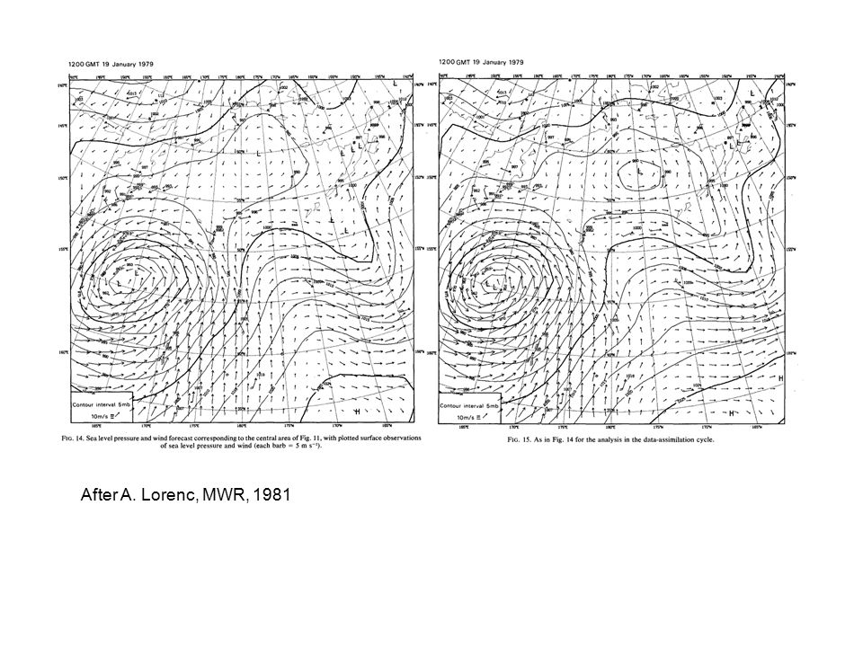
14. After A. Lorenc, MWR, 1981

16. Optimal Interpolation (continued 5) Observation vector y Estimation of a scalar x x a = E(x)  + C xy [C yy ] -1  y - E(y)  p a  E[(x-x a ) 2 ] = E(x’ 2 ) - E[(x’ a ) 2 ]) = C xx - C xy [C yy ] -1 C yx Estimation of a vector x x a = E(x)  + C xy [C yy ] -1  y - E(y)  P a  E[(x-x a ) (x-x a ) T ] = E(x’x’ T ) - E(x’ a x’ aT ) = C xx - C xy [C yy ] -1 C yx

17. Optimal Interpolation (continued 6) x a = E(x)  + C xy [C yy ] -1  y - E(y)  P a = C xx - C xy [C yy ] -1 C yx If probability distribution for couple (x, y) is Gaussian (with, in particular, covariance matrix then Optimal Interpolation achieves Bayesian estimation, in the sense that P(x | y)  N [x a, P a ]

18. Best Linear Unbiased Estimate State vector x, belonging to state space S (dim S = n), to be estimated. Available data in the form of  A ‘background’ estimate (e. g. forecast from the past), belonging to state space, with dimension n x b = x +  b  An additional set of data (e. g. observations), belonging to observation space, with dimension p y = Hx +  H is known linear observation operator. Assume probability distribution is known for the couple (  b,  ). Assume E(  b ) = 0, E(  ) = 0, E(  b  T ) = 0 (not restrictive) Set E(  b  b T ) = P b (also often denoted B), E(  T ) = R

19. Best Linear Unbiased Estimate (continuation 1) x b = x +  b (1) y = Hx +  (2) A probability distribution being known for the couple (  b,  ), eqs (1-2) define probability distribution for the couple (x, y), with E(x) = x b, x’ = x - E(x) = -  b E(y) = Hx b, y’ = y - E(y) = y - Hx b =  - H  b d  y - Hx b is called the innovation vector.

20. Best Linear Unbiased Estimate (continuation 2) Apply formulæ for Optimal Interpolation x a = x b + P b H T [HP b H T + R] -1 (y - Hx b ) P a = P b - P b H T [HP b H T + R] -1 HP b x a is the Best Linear Unbiased Estimate (BLUE) of x from x b and y. Equivalent set of formulæ x a = x b + P a H T R -1 (y - Hx b ) [P a ] -1 = [P b ] -1 + H T R -1 H Matrix K = P b H T [HP b H T + R] -1 = P a H T R -1 is gain matrix. If probability distributions are globally gaussian, BLUE achieves bayesian estimation, in the sense that P(x | x b, y) = N [x a, P a ].

21. Best Linear Unbiased Estimate (continuation 3) H can be any linear operator Example : (scalar) satellite observation x = (x 1, …, x n ) T temperature profile Observation y =  i  h i x i +  = Hx + ,  H = (h 1, …, h n ), E(  2 ) = r Backgroundx b = (x 1 b, …, x n b ) T, error covariance matrix P b = (p ij b ) x a = x b + P b H T [HP b H T + R] -1 (y - Hx b ) [HP b H T + R] -1 (y - Hx b ) = (y -   h  x  b ) / (  ij h i h j p ij b + r)   scalar !  P b = p b I n x i a = x i b + p b h i   P b = diag(p ii b ) x i a = x i b + p ii b h i   General case x i a = x i b +  j p ij b h j  Each level i is corrected, not only because of its own contribution to the observation, but because of the contribution of the other levels to which its background error is correlated.