Download presentation
Presentation is loading. Please wait.

1
Data Basics

2
Data Matrix Many datasets can be represented as a data matrix. Rows corresponding to entities Columns represents attributes. N: size of the data D: dimensionality of the data Univariate analysis: the analysis of a single attribute. Bivariate analysis: simultaneous analysis of two attributes. Multivariate analysis: simultaneous analysis of multiple attributes.

3
Example for Data Matrix

4
Attributes Categorical Attributes composed of a set of symbols has a set-valued domain E.g., Sex with domain(Sex) = {M, F}, Education with domain(Education) = { High School, BS, MS, PhD}. Two types of categorical attributes – Nominal values in the domain are unordered Only equality comparisons are allowed E.g. Sex – Ordinal Values are ordered Both equality and inequality comparisons are allowed E.g. Education

5
Attributes Cont. Numeric Attributes – Has real-valued or integer-valued domain – E.g. Age with domain (Age) = N, where N denotes the set of natural numbers (non-negative integers). Two types of numeric attributes – Discrete: values take on finite or countably infinite set. – Continuous: values take on any real value Another Classification – Interval-scaled for attributes only differences make sense E.g. temperature. – Ratio-scaled Both difference and ratios are meaningful E.g. Age
 = N, where N denotes the set of natural numbers (non-negative integers). Two types of numeric attributes – Discrete: values take on finite or countably infinite set. – Continuous: values take on any real value Another Classification – Interval-scaled for attributes only differences make sense E.g. temperature. – Ratio-scaled Both difference and ratios are meaningful E.g. Age.")
6
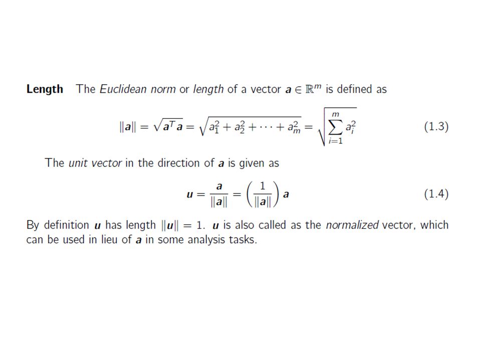
Algebraic View of Data If the d attributes in the data matrix D are all numeric each row can be considered as a d-dimensional point or equivalently, each row may be considered a d-dimensional column vector Linear combination of the standard basis vectors

7
Example of Algebraic View of Data

8
Geometric View of Data

9
Distance of Angle

12
Example of Distance and Angle

13
Mean and Total Variance

14
Centered Data Matrix The centered data matrix is obtained by subtracting the mean from all the points

15
Orthogonality Two vectors a and b are said to be orthogonal if and only if It implies that the angle between them is 90◦ or π/2 radians.

16
Orthogonal Projection P: orthogonal projection of b on the vector a; R: error vector between points b and p

17
Example of Projection

18
Linear Independence and Dimensionality : the set of all possible linear combinations of the vectors. If then we say that v1, · · ·, vk is a spanning set for.

19
Row and Column Space The column space of D, denoted col(D) is the set of all linear combinations of the d column vectors or attributes The row space of D, denoted row(D), is the set of all linear combinations of the n row vectors or points Note also that the row space of D is the column space of
 is the set of all linear combinations of the d column vectors or attributes The row space of D, denoted row(D), is the set of all linear combinations of the n row vectors or points Note also that the row space of D is the column space of")
20
Linear Independence

21
Dimension and Rank Let S be a subspace of Rm. A basis for S: a set of linearly independent vectors v1, · · ·, vk, and span(v1, · · ·, vk) = S. orthogonal basis for S: If the vectors in the basis are pair-wise orthogonal If in addition they are also normalized to be unit vectors, then they make up an orthonormal basis for S. For instance, the standard basis for Rm is an orthonormal basis consisting of the vectors
 = S. orthogonal basis for S: If the vectors in the basis are pair-wise orthogonal If in addition they are also normalized to be unit vectors, then they make up an orthonormal basis for S. For instance, the standard basis for Rm is an orthonormal basis consisting of the vectors.")
22
Any two bases for S must have the same number of vectors. Dimension: The number of vectors in a basis for S, denoted as dim(S). For any matrix, the dimension of its row and column space are the same, and this dimension is also called as the rank of the matrix.
. For any matrix, the dimension of its row and column space are the same, and this dimension is also called as the rank of the matrix..")
23
Data: Probabilistic View Assumes that each numeric attribute Xj is a random variable, defined as a function that assigns a real number to each outcome of an experiment. Given as Xj : O → R, where O, the domain of Xj, called as the sample space R, the range of Xj, is the set of real numbers. If the outcomes are numeric, and represent the observed values of the random variable, then Xj : O → O is simply the identity function: Xj (v) = v for all v ∈ O.
 = v for all v ∈ O..")
24
Data: Probabilistic View A random variable X is called a discrete random variable if it takes on only a finite or countably infinite number of values in its range. X is called a continuous random variable if it can take on any value in its range.

25
Example Be default, consider the attribute X1 to be a continuous random variable, given as the identity function X1(v) = v, since the outcomes are all numeric. On the other hand, if we want to distinguish between iris flowers with short and long sepal lengths, we define a discrete random variable A as follows In this case the domain of A is [4.3, 7.9]. The range of A is {0, 1}, and thus A assumes non-zero probability only at the discrete values 0 and 1.

27
Example: Bernoulli and Binomial Distribution only 13 irises have sepal length of at least 7cm In this case we say that A has a Bernoulli distribution with parameter p ∈ [0, 1]. p denotes the probability of a success, whereas 1− p represents the probability of a failure
![Example: Bernoulli and Binomial Distribution only 13 irises have sepal length of at least 7cm In this case we say that A has a Bernoulli distribution with parameter p ∈ [0, 1].](http://images.slideplayer.com/16/5104279/slides/slide_27.jpg "p denotes the probability of a success, whereas 1− p represents the probability of a failure.")
28
Example: Bernoulli and Binomial Distribution Let us consider another discrete random variable B, denoting the number of irises with long sepal lengths in m independent Bernoulli trials with probability of success p. B takes on the discrete values [0,m], and its probability mass function is given by the Binomial distribution For example, taking p = 0.087 from above, the probability of observing exactly k = 2 long sepal length irises in m = 10 trials is given as

29
full probability mass function for different values of k

30
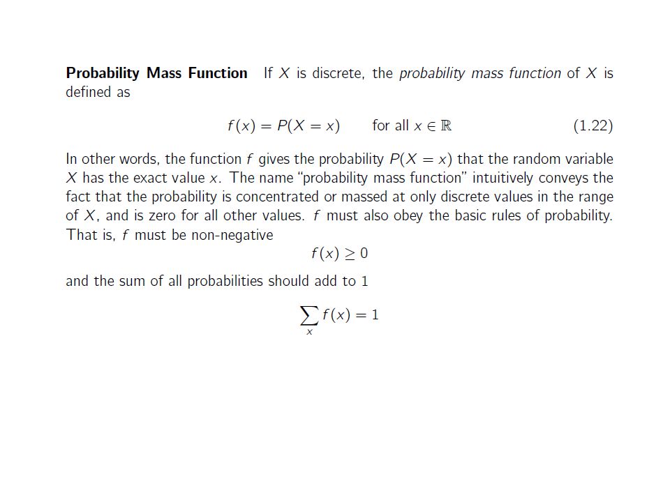
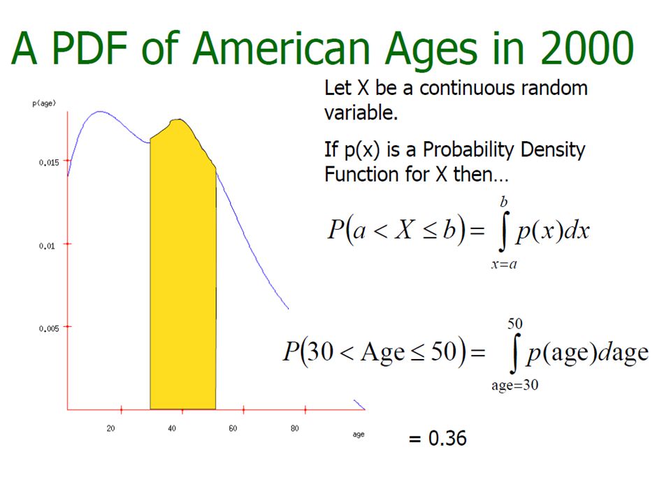
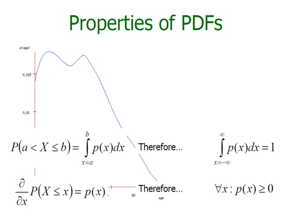
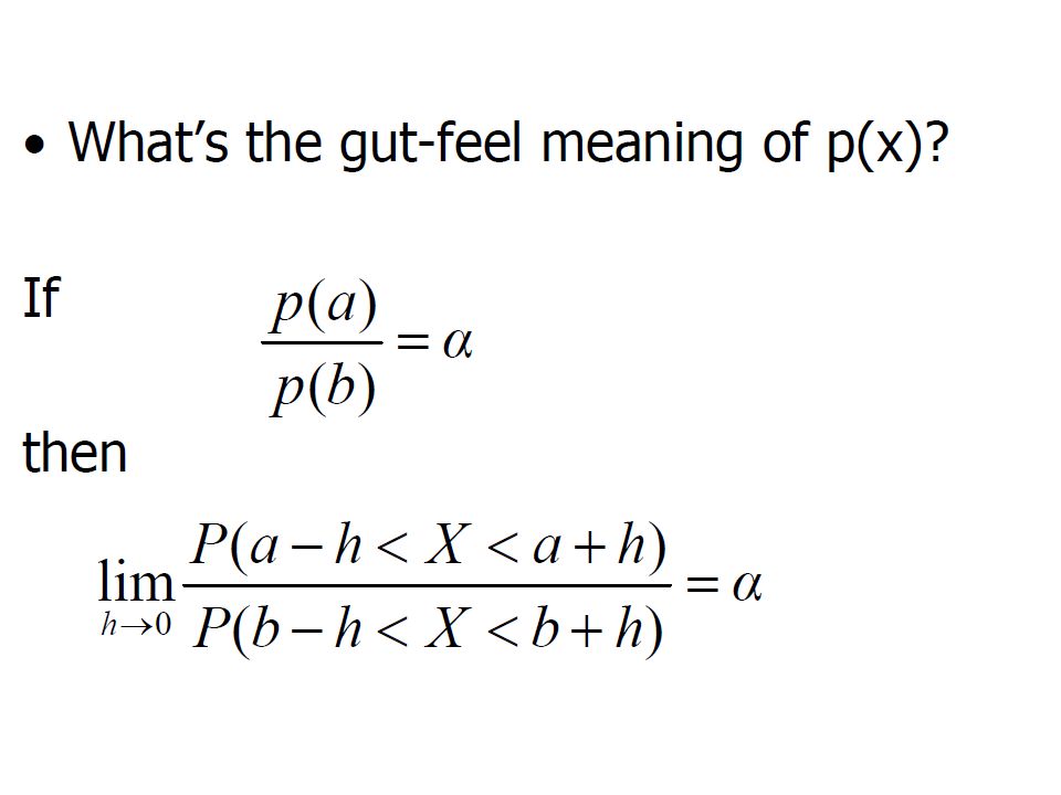
Probability Density Function If X is continuous, its range is the entire set of real numbers R. probability density function: specifies the probability that the variable X takes on values in any interval [a, b] ⊂ R

31
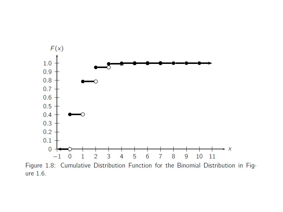
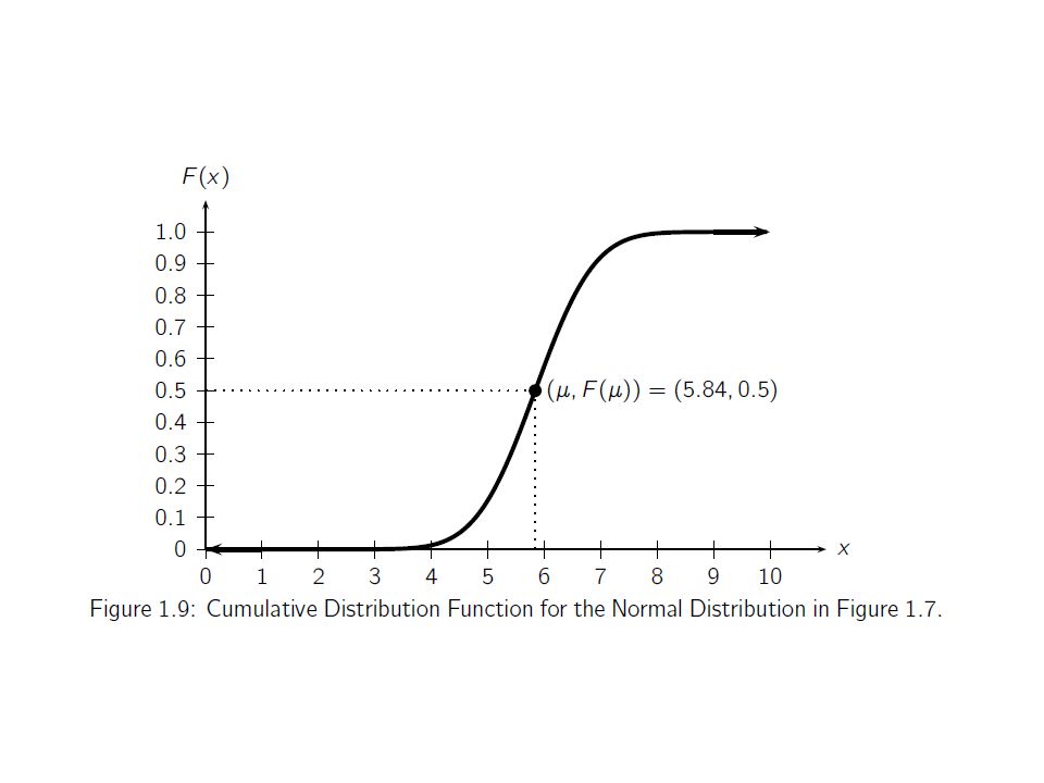
Cumulative Distribution Function For any random variable X, whether discrete or continuous, we can define the cumulative distribution function (CDF) F : R → [0, 1], that gives the probability of observing a value at most some given value x
![Cumulative Distribution Function For any random variable X, whether discrete or continuous, we can define the cumulative distribution function (CDF) F : R → [0, 1], that gives the probability of observing a value at most some given value x](http://images.slideplayer.com/16/5104279/slides/slide_31.jpg "Cumulative Distribution Function For any random variable X, whether discrete or continuous, we can define the cumulative distribution function (CDF) F : R → [0, 1], that gives the probability of observing a value at most some given value x")
33
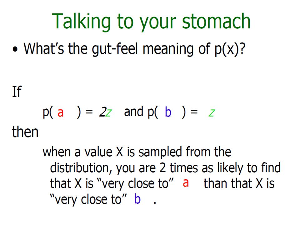
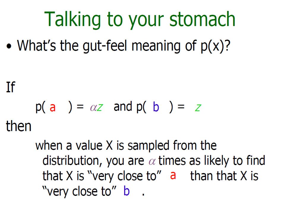
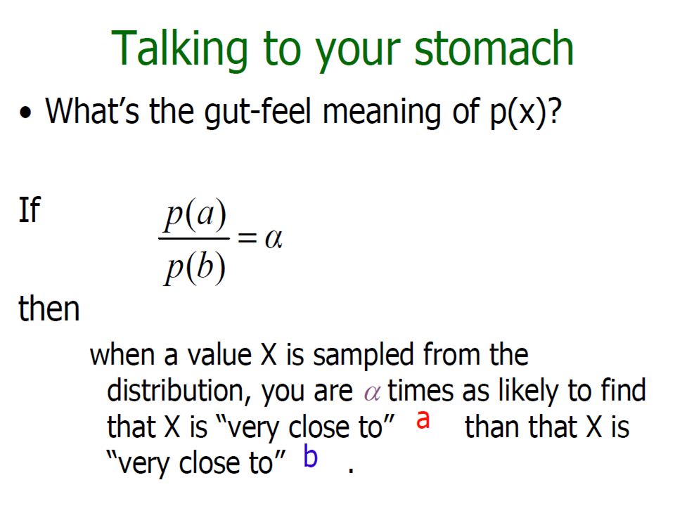
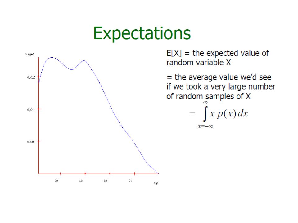
The following examples are from Andrew Moore

45
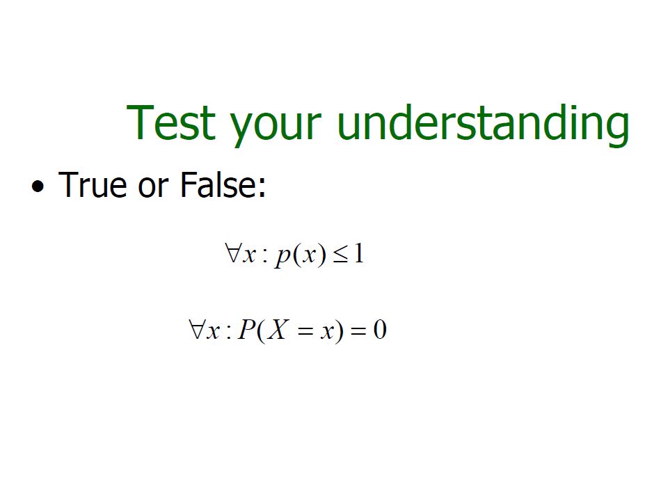
Probability Density Function f(x) What is P(X=x) when x is on a real domain » f(x) >=0 and
 What is P(X=x) when x is on a real domain » f(x) >=0 and")
46
Normal Distribution Let us assume that these values follow a Gaussian or normal density function, given as

53
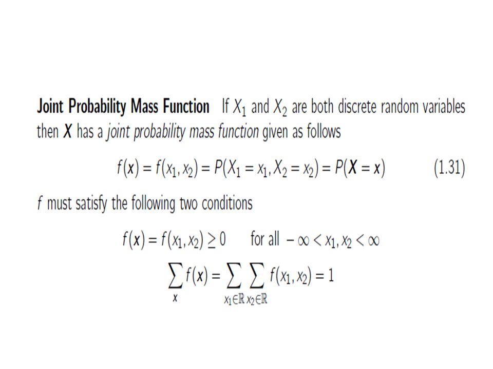
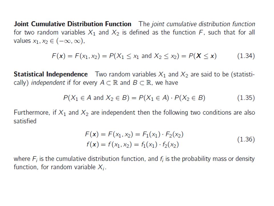
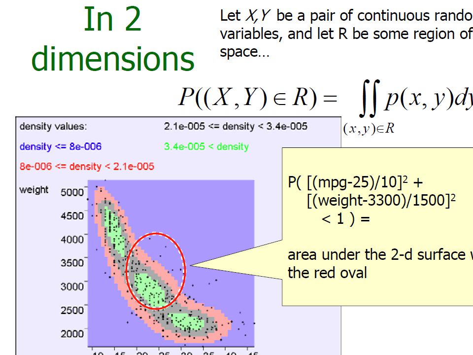
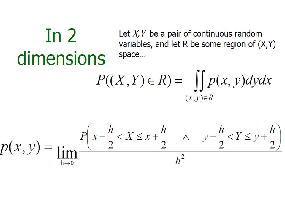
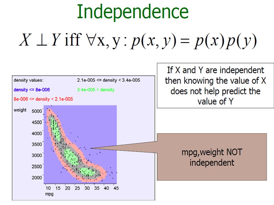
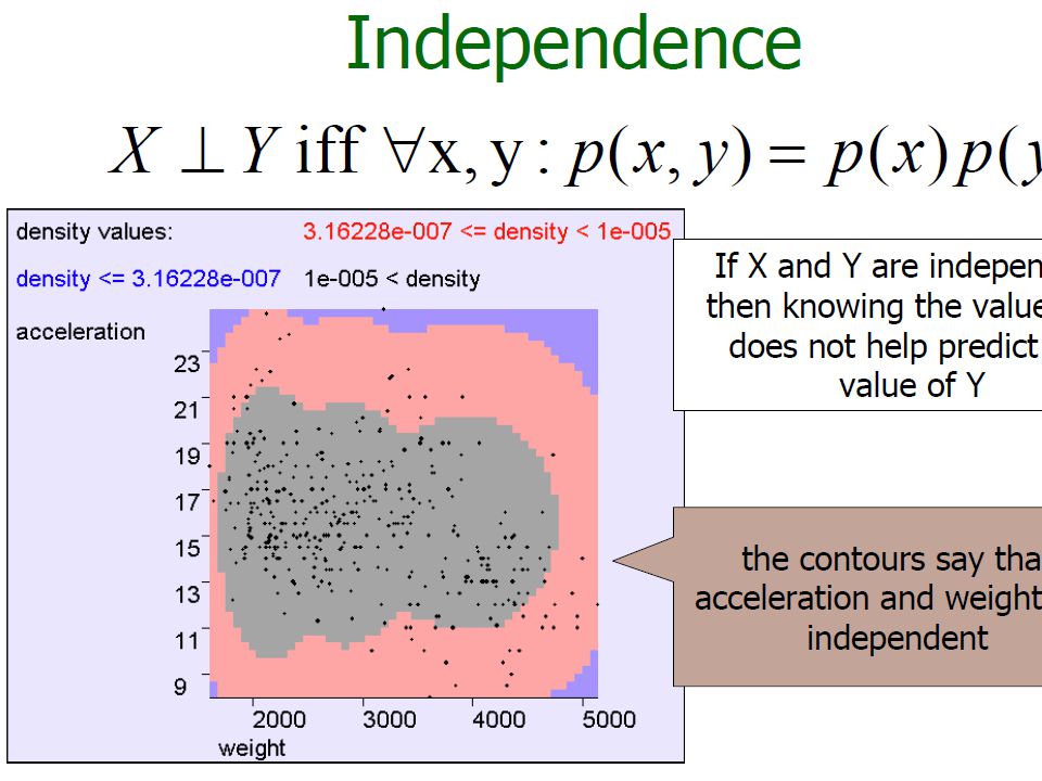
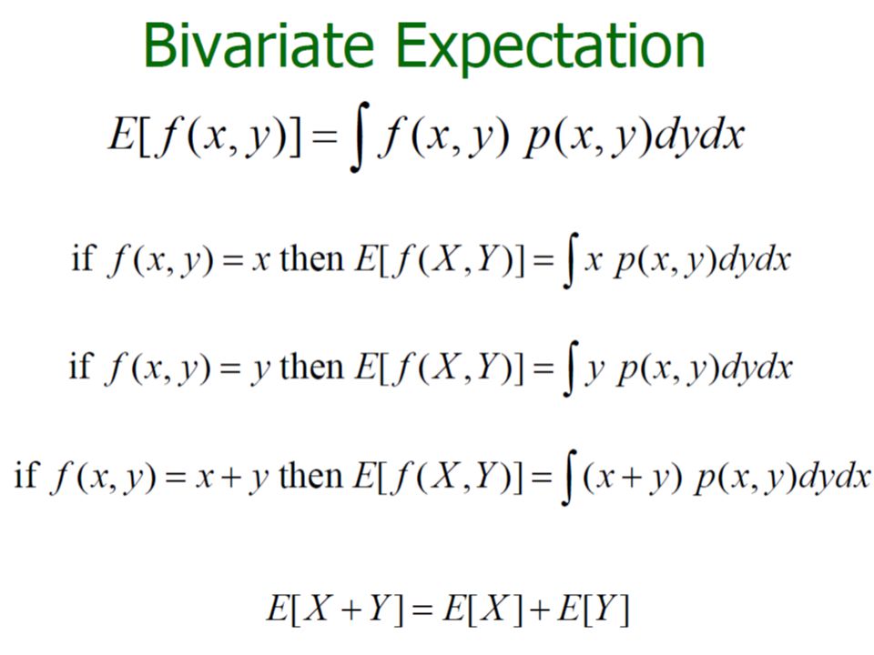
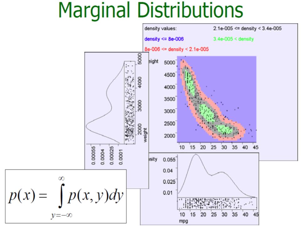
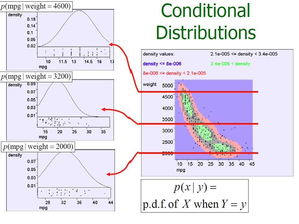
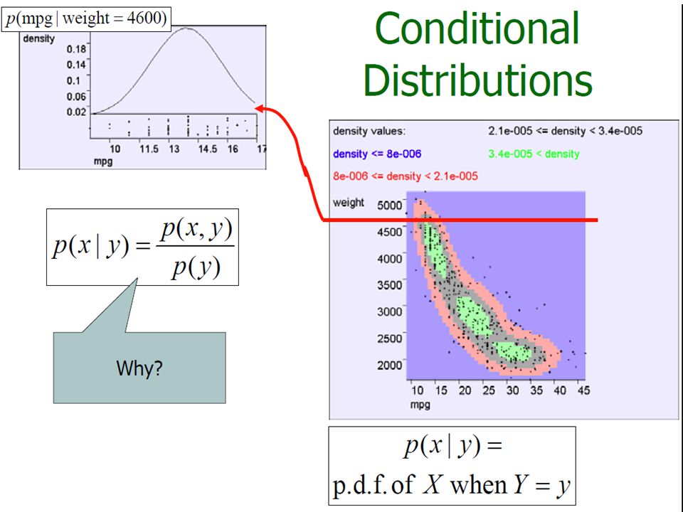
Bivariate Random Variables considering a pair of attributes, X1 and X2, as a bivariate random variable

57
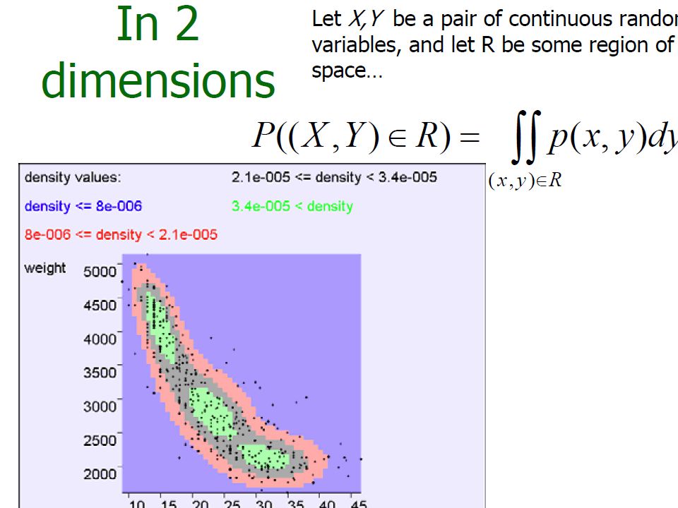
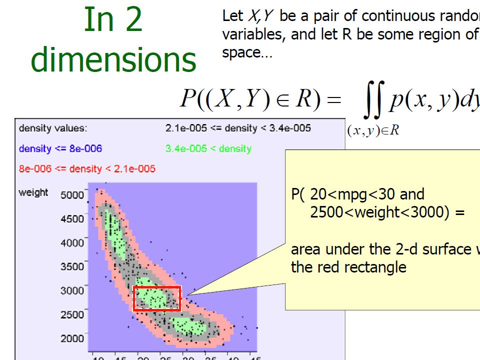
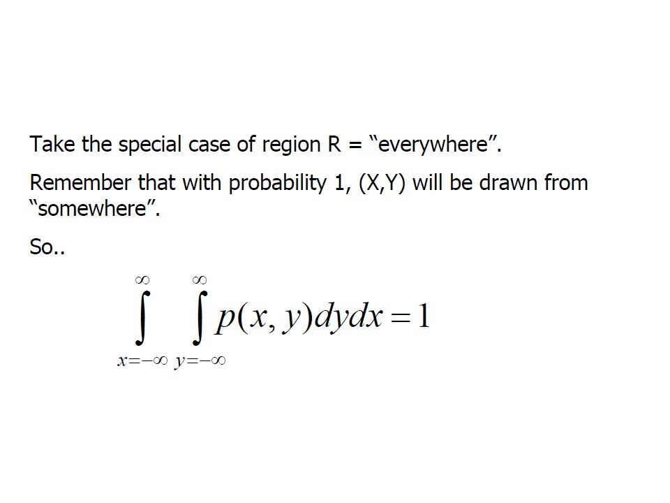
In 2-Dimensions

78
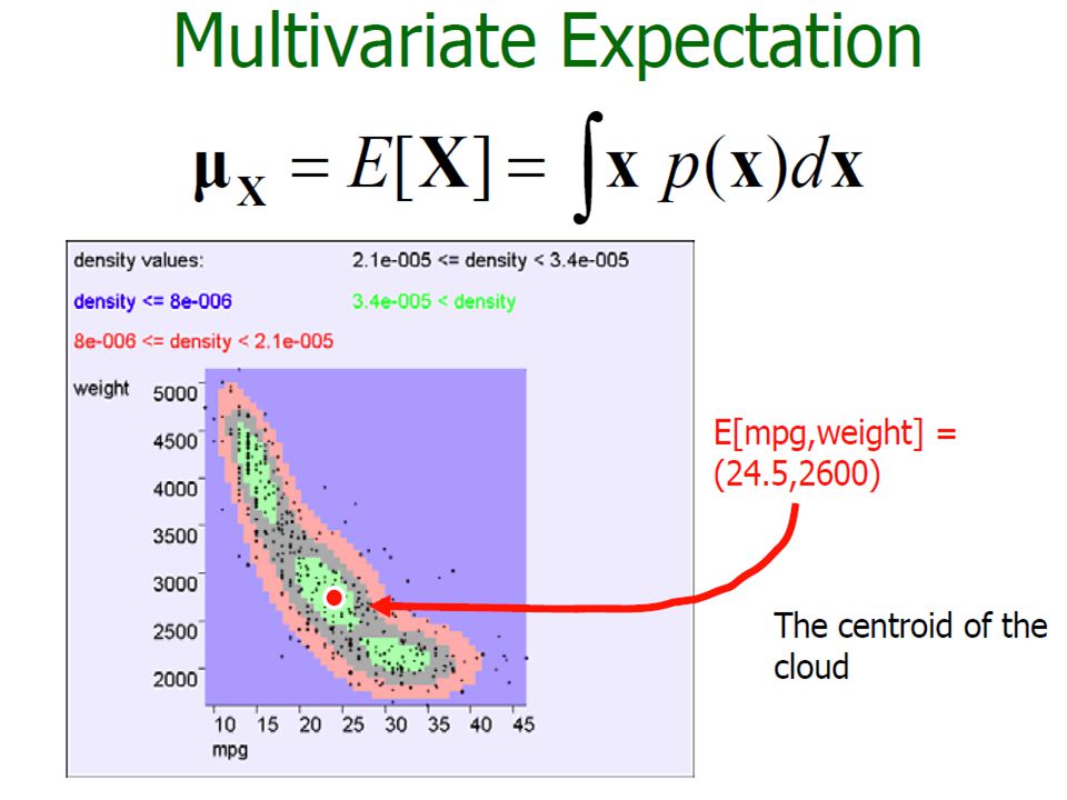
Multivariate Random Variable

80
Numeric Attribute Analysis Sample and Statistics Univariate Analysis Bivariate Analysis Multivariate Analysis Normal Distribution

81
Random Sample and Statistics Population: is used to refer to the set or universe of all entities under study. However, looking at the entire population may not be feasible, or may be too expensive. Instead, we draw a random sample from the population, and compute appropriate statistics from the sample, that give estimates of the corresponding population parameters of interest.

82
Univariate Sample Let X be a random variable, and let xi (1 ≤ i ≤ n) denote the observed values of attribute X in the given data, where n is the data size. Given a random variable X, a random sample of size n from X is defined as a set of n independent and identically distributed (IID) random variables S1, S2, · · ·, Sn. since the variables Si are all independent, their joint probability function is given as
 random variables S1, S2, · · ·, Sn. since the variables Si are all independent, their joint probability function is given as.")
83
Multivariate Sample xi: the value of a d-dimensional vector random variable Si = (X1,X2, · · ·,Xd ). Si are independent and identically distributed, and thus their joint distribution is given as Assume d attributes X1,X2, · · ·,Xd are independent, (1.43) can be rewritten as
 can be rewritten as.")
84
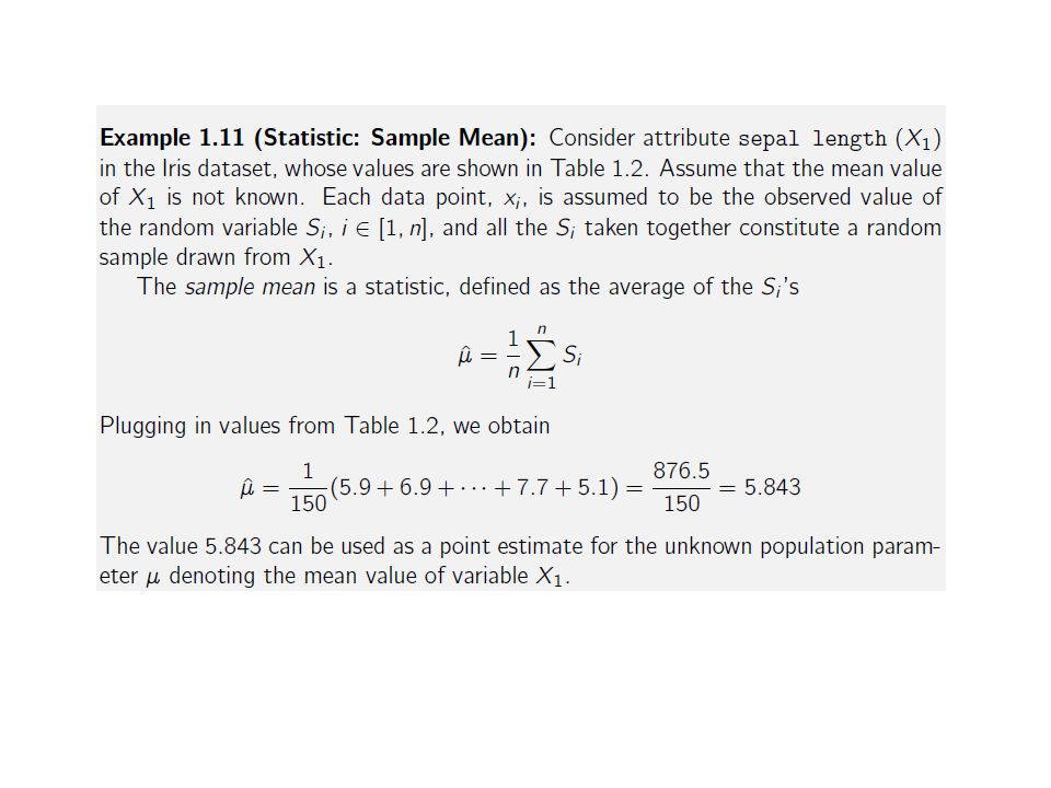
Statistic Let Si denote the random variable corresponding to data point xi, then a statistic ˆθ is a function ˆθ : (S1, S2, · · ·, Sn) → R. If we use the value of a statistic to estimate a population parameter, this value is called a point estimate of the parameter, and the statistic is called as an estimator of the parameter.

86
Numeric Attribute Analysis Sample and Statistics Univariate Analysis Bivariate Analysis Multivariate Analysis Normal Distribution

87
Univariate Analysis Univariate analysis focuses on a single attribute at a time, thus the data matrix D can be thought of as a n × 1 matrix, or simply a column vector.

88
Univariate Analysis X is assumed to be a random variable, and each point xi (1 ≤ i ≤ n) is assumed to be the value of a random variable Si, where the variables Si are all independent and identically distributed as X, i.e., they constitute a random sample drawn from X. In the vector view, we treat the sample as an n- dimensional vector, and write X ∈ Rn.

89
What can sample analysis do? Unknown f(X) and F(X) Parameters(μ,δ)
 and F(X) Parameters(μ,δ)")
90
Empirical Cumulative Distribution Function Where

91
Inverse Cumulative Distribution Function

92
Empirical Probability Mass Function Where

93
Measures of Central Tendency (Mean) Population Mean: Sample Mean (Unbiased, not robust):
 Population Mean: Sample Mean (Unbiased, not robust):")
94
Measures of Central Tendency (Median) Population Median: or Sample Median:
 Population Median: or Sample Median:")
95
Measures of Central Tendency (Mode) Sample Mode: 1. may not be very useful but not affected by the outliers too much

96
Example

97
Measures of Dispersion (Range) Range: Not robust, sensitive to extreme values Sample Range:
 Range: Not robust, sensitive to extreme values Sample Range:")
98
Measures of Dispersion (Inter-Quartile Range) Inter-Quartile Range (IQR): More robust Sample IQR:
 Inter-Quartile Range (IQR): More robust Sample IQR:")
99
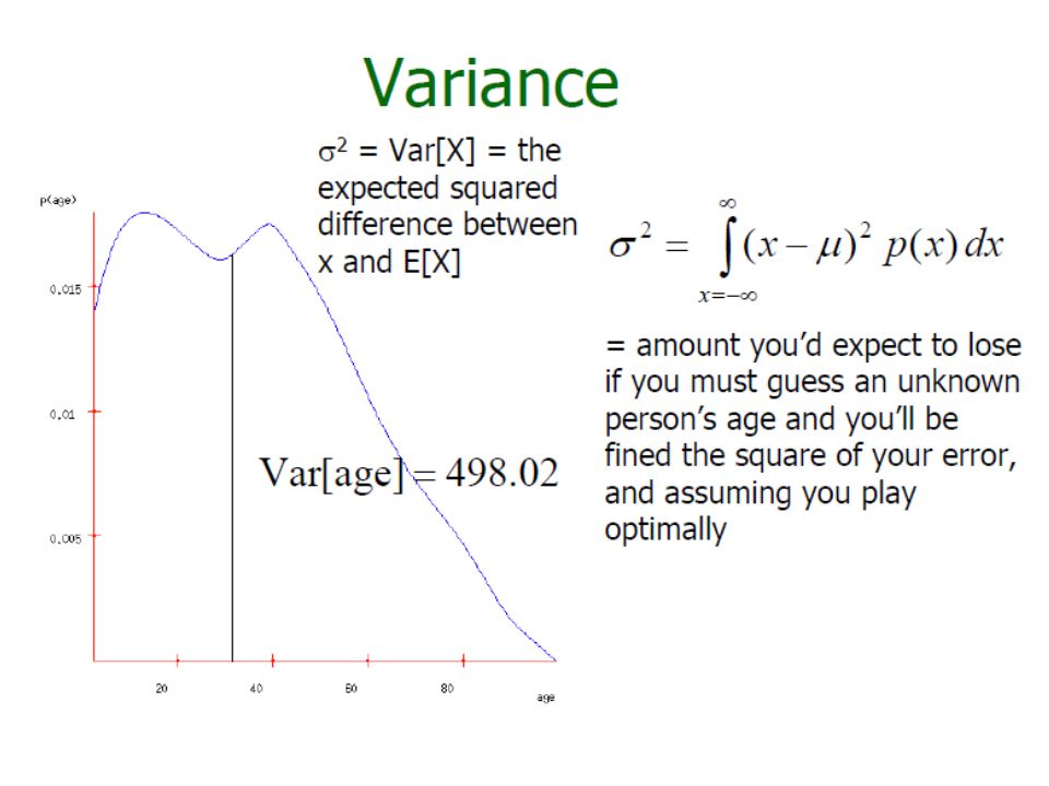
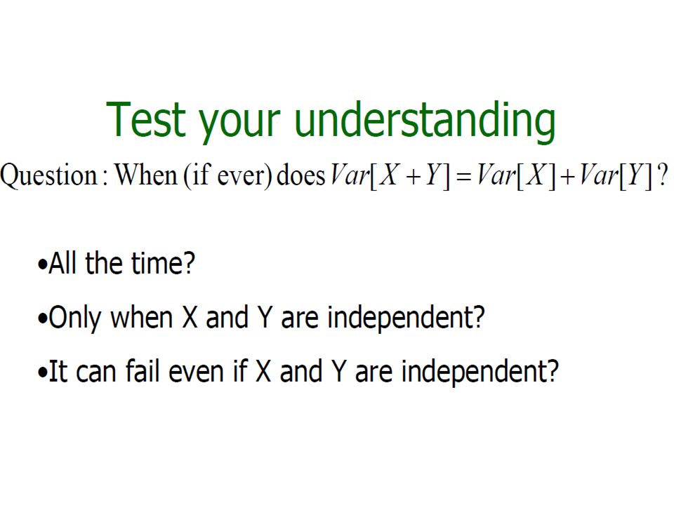
Measures of Dispersion (Variance and Standard Deviation) Standard Deviation: Variance:
 Standard Deviation: Variance:")
100
Measures of Dispersion (Variance and Standard Deviation) Standard Deviation: Variance: Sample Variance & Standard Deviation:
 Standard Deviation: Variance: Sample Variance & Standard Deviation:")
101
Normalization Z-Score: Linear Normalization:

102
Normalization Example

103
Topics Sample and Statistics Univariate Analysis Bivariate Analysis Multivariate Analysis Normal Distribution

104
Bivariate Analysis Bivariate analysis focuses on Two attributes at a time, thus the data matrix D can be thought of as a n × 2 matrix, or two column vectors.

105
Empirical Joint Probability Mass Function or where

106
Measures of Central Tendency (Mean) Population Mean: Sample Mean:
 Population Mean: Sample Mean:")
107
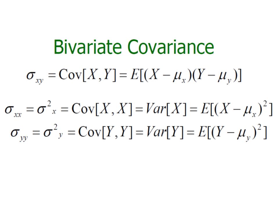
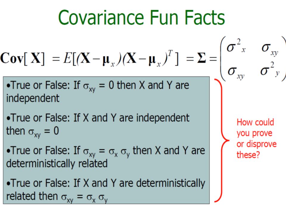
Measures of Association (Covariance) Covariance: Sample Covariance:
 Covariance: Sample Covariance:")
108
Measures of Association (Correlation) Correlation: Sample Correlation:
 Correlation: Sample Correlation:")
109
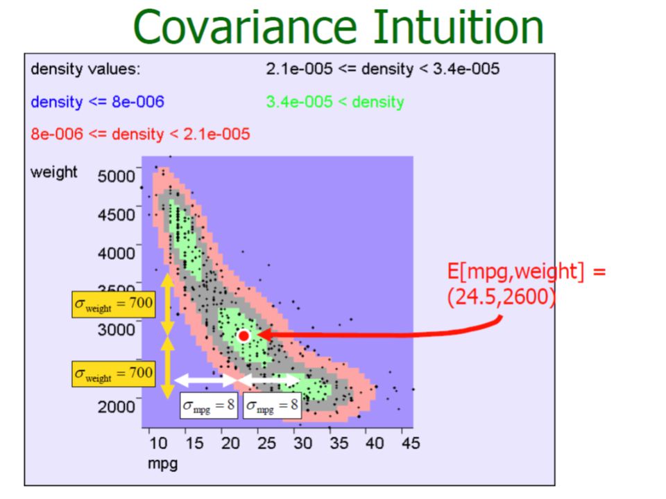
Measures of Association (Correlation)
")
110
Correlation Example

111
Topics Sample and Statistic Univariate Analysis Bivariate Analysis Multivariate Analysis Normal Distribution

112
Multivariate Analysis Multivariate analysis focuses on multiple attributes at a time, thus the data matrix D can be thought of as a n × d matrix, or d column vectors.

113
Measures of Central Tendency (Mean) Population Mean: Sample Mean:
 Population Mean: Sample Mean:")
114
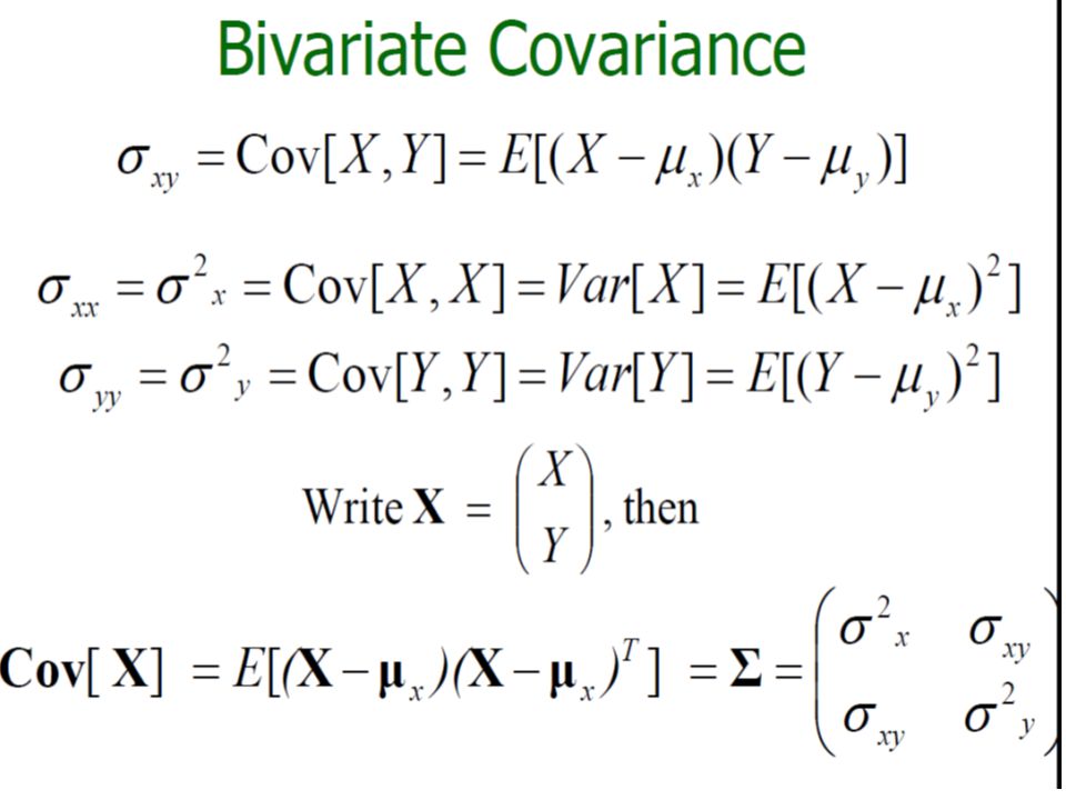
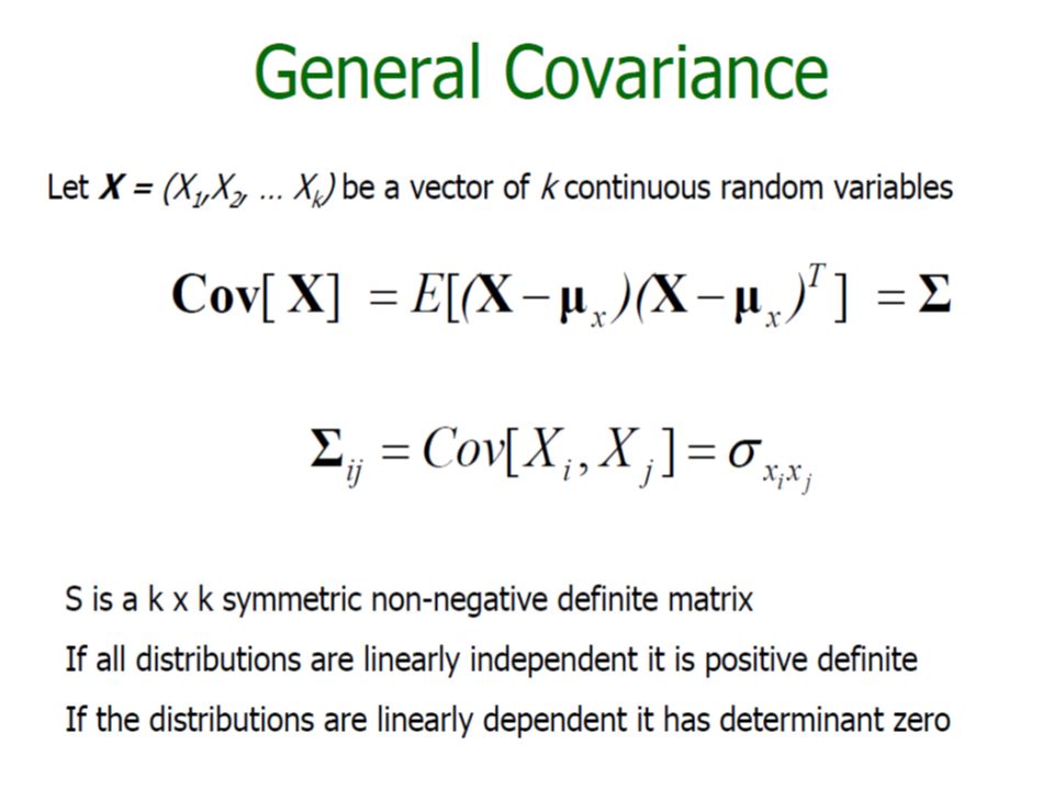
Measures of Association (Covariance Matrix)
")
115
Measures of Association (Correlation) Correlation: Sample Correlation:
 Correlation: Sample Correlation:")
116
Topics Sample and Statistic Univariate Analysis Bivariate Analysis Multivariate Analysis Normal Distribution

117
Univariate Normal Distribution

118
Multivariate Normal Distribution

119
Thank You!

Similar presentations