1. Diffusion Over Dynamic Networks Stanford University May 8, 2007 James Moody Duke University

2. Introduction We live in a connected world: “To speak of social life is to speak of the association between people – their associating in work and in play, in love and in war, to trade or to worship, to help or to hinder. It is in the social relations men establish that their interests find expression and their desires become realized.” Peter M. Blau Exchange and Power in Social Life, 1964

3. Introduction These patterns of connection form a social space, that can be seen in multiple contexts: We live in a connected world: "If we ever get to the point of charting a whole city or a whole nation, we would have … a picture of a vast solar system of intangible structures, powerfully influencing conduct, as gravitation does in space. Such an invisible structure underlies society and has its influence in determining the conduct of society as a whole." J.L. Moreno, New York Times, April 13, 1933

4. Source: Linton Freeman “See you in the funny pages” Connections, 23, 2000, 32-42. Introduction

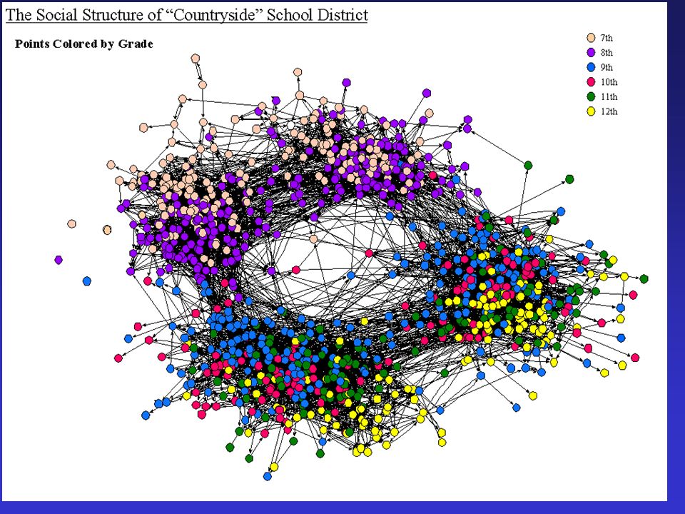
5. High Schools as Networks Introduction

8. And yet, standard social science analysis methods do not take this space into account. “For the last thirty years, empirical social research has been dominated by the sample survey. But as usually practiced, …, the survey is a sociological meat grinder, tearing the individual from his social context and guaranteeing that nobody in the study interacts with anyone else in it.” Allen Barton, 1968 (Quoted in Freeman 2004) Moreover, the complexity of the relational world makes it impossible to identify social connectivity using only our intuitive understanding. Social Network Analysis (SNA) provides a set of tools to empirically extend our theoretical intuition of the patterns that construct social structure. Introduction

9. Why do Networks Matter?Local vision Introduction

10. Why do Networks Matter?Local vision Introduction

11. Why networks matter: Intuitive: “goods” travel through contacts between actors, which can reflect a power distribution or influence attitudes and behaviors. Our understanding of social life improves if we account for this social space. Less intuitive: patterns of inter-actor contact can have effects on the spread of “goods” or power dynamics that could not be seen focusing only on individual behavior. These, ultimately, are often features that rest on the diffusion of some “bit” over the network. We’ll focus today on how that happens. Introduction

12. Social Network Data Elements Social Network data consists of two linked classes of data: a)Information on the individuals (aka: actors, nodes, points) Network nodes are most often people, but can be any other unit capable of being linked to another (schools, countries, organizations, personalities, etc.) The information about nodes is what we usually collect in standard social science research: demographics, attitudes, behaviors, etc. Includes the times when the node is active b) Information on relations among individuals (lines, edges, arcs) Records a connection between the nodes in the network Can be valued, directed (arcs), binary or undirected (edges) One-mode (direct ties between actors) or two-mode (actors share membership in an organization) Includes the times when the relation is active

13. In general, a relation can be: Binary or Valued Directed or Undirected a b ce d Undirected, binary Directed, binary a b ce d a b ce d Undirected, Valued Directed, Valued a b ce d 13 4 2 1 Social Network Data Elements

14. “Goods” flow through networks: Social Networks & Diffusion

15. In addition to* the dyadic probability that one actor passes something to another (p ij ), two factors affect flow through a network: Topology -the shape, or form, of the network - Example: one actor cannot pass information to another unless they are either directly or indirectly connected Time - the timing of contact matters - Example: an actor cannot pass information he has not receive yet Social Networks & Diffusion *This is a big conditional! – lots of work on how the dyadic transmission rate may differ across populations.

16. Three features of the network’s topology are known to be important: Reachability, Distance & Number of Paths (redundancy) Connectivity refers to how actors in one part of the network are connected to actors in another part of the network. Reachability: Is it possible for actor i to reach actor j? This can only be true if there is a chain of contact from one actor to another. Distance: Given they can be reached, how many steps are they from each other? How efficiently do ties reach new nodes? (How clustered is the network) Number of paths: How many different paths connect each pair? Social Networks & Diffusion

17. Without full network data, you can’t distinguish actors with limited diffusion potential from those more deeply embedded in a setting. a b c Social Networks & Diffusion

18. Reachability Given that ego can reach alter, distance determines the likelihood of information passing from one end of the chain to another. Because flow is rarely certain, the probability of transfer decreases over distance. However, the probability of transfer increases with each alternative path connecting pairs of people in the network. Social Networks & Diffusion

19. d e c Indirect connections are what make networks systems. One actor can reach another if there is a path in the graph connecting them. a b ce d f bf a Reachability Paths can be directed, leading to a distinction between “strong” and “weak” components Social Networks & Diffusion

20. Basic elements in connectivity A path is a sequence of nodes and edges starting with one node and ending with another, tracing the indirect connection between the two. On a path, you never go backwards or revisit the same node twice. Example: a  b  c  d A walk is any sequence of nodes and edges, and may go backwards. Example: a  b  c  b  c  d A cycle is a path that starts and ends with the same node. Example: a  b  c  a Reachability Social Networks & Diffusion

21. Reachability If you can trace a sequence of relations from one actor to another, then the two are reachable. If there is at least one path connecting every pair of actors in the graph, the graph is connected and is called a component. Intuitively, a component is the set of people who are all connected by a chain of relations. Reachability Social Networks & Diffusion

22. This example contains many components. Reachability Social Networks & Diffusion

23. a Distance is measured by the (weighted) number of relations separating a pair: Actor “a” is: 1 step from 4 2 steps from 5 3 steps from 4 4 steps from 3 5 steps from 1 Distance & number of paths Social Networks & Diffusion

24. Paths are the different routes one can take. Node-independent paths are particularly important. a b There are 2 independent paths connecting a and b. There are many non- independent paths Distance & number of paths Social Networks & Diffusion

25. White, D. R. and F. Harary. 2001. "The Cohesiveness of Blocks in Social Networks: Node Connectivity and Conditional Density." Sociological Methodology 31:305-59. Moody, James and Douglas R. White. 2003. “Structural Cohesion and Embeddedness: A hierarchical Conception of Social Groups” American Sociological Review 68:103-127 White, Douglas R., Jason Owen-Smith, James Moody, & Walter W. Powell (2004) "Networks, Fields, and Organizations: Scale, Topology and Cohesive Embeddings." Computational and Mathematical Organization Theory. 10:95-117 Moody, James "The Structure of a Social Science Collaboration Network: Disciplinary Cohesion from 1963 to 1999" American Sociological Review. 69:213- 238 Social Cohesion Social Networks & Diffusion

26. Networks are structurally cohesive if they remain connected even when nodes are removed. Each of these graphs have the exact same density. Node Connectivity 01 23 Social Cohesion Social Networks & Diffusion

27. Formal definition of Structural Cohesion: (a)A group’s structural cohesion is equal to the minimum number of actors who, if removed from the group, would disconnect the group. Equivalently (by Menger’s Theorem): (b)A group’s structural cohesion is equal to the minimum number of node- independent paths linking each pair of actors in the group. Social Cohesion Social Networks & Diffusion

28. Structural cohesion gives rise automatically to a clear notion of embeddedness, since cohesive sets nest inside of each other. 17 18 19 20 2 22 23 8 11 10 14 12 9 15 16 13 4 1 75 6 3 2 Social Cohesion Social Networks & Diffusion

29. 3-Component (n=58) Project 90, Sex-only network (n=695) Social Cohesion Social Networks & Diffusion

30. Connected Bicomponents IV Drug Sharing Largest BC: 247 k > 4: 318 Max k: 12 Structural Cohesion simultaneously gives us a positional and subgroup analysis. Social Cohesion Social Networks & Diffusion

31. Partner Distribution Component Size/Shape Emergent Connectivity in low-degree networks Social Networks & Diffusion Emergence of multiple connectivity by degree distribution

32. Development of STD cores in low-degree networks: rapid transition without stars. Social Networks & Diffusion Emergence of multiple connectivity by degree distribution

33. Probability of transfer by distance and number of paths, assume a constant p ij of 0.6 0 0.2 0.4 0.6 0.8 1 1.2 23456 Path distance probability 10 paths 5 paths 2 paths 1 path Distance & number of paths Social Networks & Diffusion

34. Clustering and diffusion Arcs: 11 Largest component: 12, Clustering: 0 Arcs: 11 Largest component: 8, Clustering: 0.205 Clustering turns network paths back on already identified nodes. This has been well known since at least Rappaport, and is a key feature of the “Biased Network” models in sociology.

35. Social Networks & Diffusion Diffusion features on static graphs

36. Social Networks & Diffusion Example on static graphs

37. Social Networks & Diffusion Example on static graphs Define as a general measure of the “diffusion susceptibility” of a graph as the ratio of the area under the observed curve to the area under the random curve. As this gets smaller than 1.0, you get effectively slower median transmission.

38. Social Networks & Diffusion Example on static graphs

39. Social Networks & Diffusion Example on static graphs

40. Centrality refers to (one dimension of) location, identifying where an actor resides in a network. For example, we can compare actors at the edge of the network to actors at the center. In general, this is a way to formalize intuitive notions about the distinction between insiders and outsiders. Centrality affects within-network diffusion likelihood – we’ll not talk about this much today. Centrality Social Networks & Diffusion

41. At the individual level, one dimension of position in the network can be captured through centrality. Conceptually, centrality is fairly straight forward: we want to identify which nodes are in the ‘center’ of the network. In practice, identifying exactly what we mean by ‘center’ is somewhat complicated, but substantively we often have reason to believe that people at the center are very important. Three standard centrality measures capture a wide range of “importance” in a network: Degree Closeness Betweenness Centrality Social Networks & Diffusion

42. A common measure of centrality is closeness centrality. An actor is considered important if he/she is relatively close to all other actors. Closeness is based on the inverse of the distance of each actor to every other actor in the network. Closeness Centrality: Normalized Closeness Centrality Centrality Social Networks & Diffusion

43. Closeness Centrality in 4 examples C=1.0 C=0.0 C=0.36 C=0.28 Centrality Social Networks & Diffusion

44. Two factors that affect network flows: Topology - the shape, or form, of the network - simple example: one actor cannot pass information to another unless they are either directly or indirectly connected Time - the timing of contacts matters - simple example: an actor cannot pass information he has not yet received. Time Measuring Networks: Flow

45. Timing in networks A focus on contact structure has often slighted the importance of network dynamics,though a number of recent pieces are addressing this. Time affects networks in two important ways: 1)The structure itself evolves, in ways that will affect the topology an thus flow. 2) The timing of contact constrains information flow Time Measuring Networks: Flow

46. Data on drug users in Colorado Springs, over 5 years Drug Relations, Colorado Springs, Year 1 Time Measuring Networks: Flow

47. Drug Relations, Colorado Springs, Year 2 Current year in red, past relations in gray Time Measuring Networks: Flow

48. Drug Relations, Colorado Springs, Year 3 Current year in red, past relations in gray Time Measuring Networks: Flow

49. Drug Relations, Colorado Springs, Year 4 Current year in red, past relations in gray Time Measuring Networks: Flow

50. Drug Relations, Colorado Springs, Year 5 Current year in red, past relations in gray Time Measuring Networks: Flow

51. When is a network? Source: Bender-deMoll & McFarland “The Art and Science of Dynamic Network Visualization ” JoSS 2006

52. When is a network? At the finest levels of aggregation networks disappear, but at the higher levels of aggregation we mistake momentary events as long-lasting structure. Is there a principled way to analyze and visualize networks where the edges are not stable? There is unlikely to be a single answer for all questions, but the set of types of questions might be manageable: Diffusion and flow (networks as resources or constraints for actors): The timing of relations affects flow in a way that changes many of our standard measures. If our interest is in “Relational ties [as] channels for transfer or flow of resources” (W&F p.4), then we can use the diffusion process to shape our analyses. Structural change (networks as dynamic objects of study). The interest is in mapping changes in the topography of the network, to see model how the field itself changes over time. Ultimately, this has to be linked to questions about how network macro- structures emerge as the result of actor behavior rules.

53. Network Dynamics & Flow The key element that makes a network a system is the path: it’s how sets of actors are linked together indirectly. A walk is a sequence of nodes and lines, starting and ending with nodes, in which each node is incident with the lines following and preceding it in a sequence. A path is a walk where all of the nodes and lines are distinct. Paths are the routes through networks that make diffusion possible. In a dynamic network, the timing of edges affect whether a good can flow across a path. A good cannot pass along a relation that ends prior to the actor receiving the good: goods can only flow forward in time. A time-ordered path exists between i and j if a graph-path from i to j can be identified where the starting time for each edge step precedes the ending time for the next edge. The notion of a time-ordered path must change our understanding of the system structure of the network. Networks exist both in relation-space and time-space.

54. Network Dynamics & Flow A time-ordered path exists between i and j if a graph-path from i to j can be identified where the starting time for each edge step precedes the ending time for the next edge. Note that this allows for non-intuitive non-transitivity. Consider this simple example: Here A can reach B, B can reach C, and C and reach D. But A cannot reach D, since any flow from A to C would have happened after the relation between C and D ended. ABC D 1 - 2 3 - 4 1 - 2

55. Network Dynamics & Flow This can also introduce a new dimension for “shortest” paths: A BC D 1 - 2 3 - 4 5 - 6 E 7 - 9 The geodesic from A to D is AE, ED and is two steps long. But the fastest path would be AB, BC, CD, which while 3 steps long could get there by day 5 compared to day 7.

56. B C E DF A 2 - 5 3 - 7 0 - 1 8 - 9 3 - 5 A hypothetical Sexual Contact Network Edge timing constraints on diffusion “Bits” can only flow forward in time: the finish time of the next step in a path must be > the start time of the last step.

57. The path graph for a hypothetical contact network Edge timing constraints on diffusion “Bits” can only flow forward in time: the finish time of the next step in a path must be > the start time of the last step. B C E DF A

58. Edge timing constraints on diffusion Edge time structures are characterized by sequence, duration and overlap. Paths between i and j, have length and duration, but these need not be symmetric even if the constituent edges are symmetric.

59. Direct Contact Network of 8 people in a ring Network Dynamics & Flow Reachability

60. Implied Contact Network of 8 people in a ring All relations Concurrent Network Dynamics & Flow Reachability

61. Implied Contact Network of 8 people in a ring Mixed Concurrent 2 2 1 1 2 2 3 3 Network Dynamics & Flow = 0.57 reachability Reachability

62. Implied Contact Network of 8 people in a ring Serial Monogamy (1) 1 2 3 7 6 5 8 4 Network Dynamics & Flow = 0.71 reachability Reachability

63. Implied Contact Network of 8 people in a ring Serial Monogamy (2) 1 2 3 7 6 1 8 4 Network Dynamics & Flow = 0.51 reachability Reachability

64. Minimum Contact Network of 8 people in a ring Serial Monogamy (3) 1 2 1 1 2 1 2 2 Network Dynamics & Flow = 0.43 reachability Which is the minimum possible reachability given the contact structure.

65. 1 2 1 1 2 1 2 2 Network Dynamics & Flow In this graph, timing alone can change mean reachability from 2.0 when all ties are concurrent to 0.43: a factor of ~ 4.7. In general, ignoring time order is equivalent to assuming all relations occur simultaneously – assumes perfect concurrency across all relations.

66. Edge timing constraints on diffusion A B C D E F A 0 1 2 2 4 1 B 1 0 1 2 3 2 C 0 1 0 1 2 2 D 0 0 1 0 1 1 E 0 0 0 1 0 2 F 1 0 0 1 0 0 Path distances need not progress in steps. While (a) is 2 steps from d, and d is 1 step from e, a and e are 4 steps apart. This is because a shorter path from a to e emerges after the path from d to e ended. 4 2 1

67. 1 2 1 1 2 1 2 2 Network Dynamics & Flow At the graph level, we are interested in two properties immediately: a)the temporal-implied reachability (perhaps relative to minimum) b) The asymmetry in reachability. What proportion of reachable dyads can mutually reach each other? These are directly relevant for overall diffusion potential in a network.

68. Network Dynamics & Flow The distribution of paths is important for many of the measures we typically construct on networks, and these will be change if timing is taken into consideration: Centrality: Closeness centrality Path Centrality Information Centrality Betweenness centrality Network Topography Clustering Path Distance Groups & Roles: Correspondence between degree-based position and reach-based position Structural Cohesion & Embeddedness Opportunities for Time-based block-models (similar reachability profiles) In general, any measures that take the systems nature of the graph into account will differ in a dynamic graph from a static graph.

69. Network Dynamics & Flow New versions of classic reachability measures: 1)Temporal reach: The ij cell = 1 if i can reach j through time. 2)Temporal geodesic: The ij cell equals the number of steps in the shortest path linking i to j over time. 3)Temporal cohesion: The ij cell equals the number of time-ordered node- independent paths linking i to j. These will only equal the standard versions when all ties are concurrent. Duration explicit measures 4) Quickest path: The ij cell equals the shortest time within which i could reach j. 5) Earliest path: The ij cell equals the real-clock time when i could first reach j. 6) Latest path: The ij cell equals the real-clock time when i could last reach j. 7) Exposure duration: The ij cell equals the longest (shortest) interval of time over which i could transfer a good to j. Each of these also imply different types of “betweenness” roles for nodes or edges, such as a “limiting time” edge, which would be the edge whose comparatively short duration places the greatest limits on other paths.

70. Network Dynamics & Flow Define time-dependent closeness as the inverse of the sum of the distances needed for an actor to reach others in the network. * Actors with high time-dependent closeness centrality are those that can reach others in few steps given temporal order. Note this is directed. Since D ij =/= D ji (in most cases) once you take time into account. * If i cannot reach j, I set the distance to n+1

71. Network Dynamics & Flow Define fastness centrality as the average of the clock-time needed for an actor to reach others in the network: Actors with high fastness centrality are those that would reach the most people early. These are likely important for any “first mover” problem.

72. Network Dynamics & Flow Define quickness centrality as the average of the minimum amount of time needed for an actor to reach others in the network: Where T jit is the time that j receives the good sent by i at time t, and T it is the time that i sent the good. This then represents the shortest duration between transmission and receipt between i and j. Note that this is a time-dependent feature, depending on when i “transmits” the good out into the population. The min is one of many functions, since the time-to-target speed is really a profile over the duration of t.

73. Network Dynamics & Flow Define exposure centrality as the average of the amount of time that actor j is at risk to a good introduced by actor i. Where T ijl is the last time that j could receive the good from i and T iif is the first time that j could receive the good from i, so the difference is the interval in time when i is at risk from j.

74. Network Dynamics & Flow How do these centrality scores compare to static scores? Here I compare the duration-dependent measures to the standard measures on this example graph. Based only on the structure of the ties, not the timing, the most central nodes are nodes 13, 16 and 4. Since this is a simulation, I simply randomize the observed time-ranges on this graph to test the general relation between the fixed and temporal measures.

75. Network Dynamics & Flow How do these centrality scores compare to static scores? Here I compare the duration-dependent measures to the standard measures on this example graph. Box plots based on 500 permutations of the observed time durations. This holds constant the duration distribution and the number of edges active at any given time.

76. Network Dynamics & Flow How do these centrality scores compare? What about at the system level? How do the features of the temporal ordering affect the overall asymmetry in reachability and the proportion of pairs reachable? Reachability Asymmetry Concordance (  3 )

77. Network Dynamics & Flow How do these centrality scores compare? The “most important actors” in the graph depend crucially on when they are active. The correlations can range wildly over the exact same contact structure. Concordance is important, but not determinant (at least within the range studied here). We need to extend our intuition on the global distribution of time in the graph. The “centrality” scores described here are low-hanging fruit: simple extensions of graph-based ideas. But the crucial features for population interests will be creating aggregations of these features – something like “centralization” that captures the regularity, asymmetry and temporal role-structure of the network.

78. The Cocktail Party Problem -Imagine a typical ‘mixer’ party, where one of the guests knows a bit of gossip that everyone would like to know. -Assuming that people tell this gossip to the people they meet at the party: a)How many people would eventually hear the gossip? b)How long would it take to spread through the group?

79. The Cocktail Party Problem -Some specifics to narrow down the problem. - 30 people invited, party lasts an hour. -At any given moment in time, you can only carry on a conversation with 3 other people -Guests mingle well – they spend a short time talking to most people, but a long time to a small number (such as their date). -Mingling is somewhat space-based – you talk to the people you bump into, then move on to someone else after a short time. -The bit of gossip moves instantaneously across connected sets (so time-to-diffuse=0).

80. The Cocktail Party Problem -Some specifics to narrow down the problem. A (seemingly) simple network problem: record who talks to who, and map the network. Mean distance: 1.99 Diameter: 4 steps

81. The Cocktail Party Problem -But such an image conflates many temporally distinct events. A more accurate image is something like this: In general, the graphs over which diffusion happens often: Have timed edges Nodes enter and leave Edges can re-occur multiple times Edges can be concurrent These features break transmission paths, generally lowering diffusion potential – and opening a host of interesting questions about the intersection of structure and time in networks.

82. The Party Revisited Question 1: How does the edge timing affect the overall likelihood that everyone in the party would ultimately hear the gossip? Simulate a cocktail party, manipulate the “mingling” rate and range and compare diffusion over both networks.

83. The Party Revisited

84. Sample “traces” from one run Measuring Diffusion Potential with Network Traces: Cumulative Number of people each node reaches at each step. Static Graph Node reaches 9 people in 2 steps Nodes that reach everyone in 4 steps Dynamic Graph Nodes that never reach everyone

85. The Party Revisited Average (mean of means) reachability & Distance, all runs Static Density: 0.42 Static Density: 0.21 Static Density: 0.23 Static Density: 0.27 Static Density: 0.30 Static Density: 0.24 Static Density: 0.27 Static Density: 0.32 Static Density: 0.34 Static Density: 0.26 Static Density: 0.31 Static Density: 0.35 Static Density: 0.41 Static Density: 0.28 Static Density: 0.36 Static Density: 0.40

86. The Party Revisited Timing always lowers the proportion who could be reached in the network and lengthens the distances between connected nodes. This suggests that diffusion over dynamic networks will tend to be slower than over similar volume static nets. Note that here we: a) assumed that diffusion was instant across connected sets b) assumed complete cliques among conversation groups c) everyone started at the same time d) a small group (30 nodes). If the group is larger, the proportional effects are more dramatic. If diffusion takes time, edges expire before traversed. Question 2: Since old paths can’t be joined when actors make new contacts, will the “small world” rewiring effect work?

87. Small World Mechanisms on Dynamic Graphs

88. Concurrency opens paths for diffusion to move reciprocally. Small World Mechanisms on Dynamic Graphs Use concurrency to adjust the temporal structure of the graph.

89. Small World Mechanisms on Dynamic Graphs Simulation setup: 1.Generate a 200 node ring lattice, where every node has 6 ties. 2.Assign starting times to edges as a random draw from a uniform distribution. Mean concurrency levels are set by compressing or stretching the starting-time distribution. 3.Each edge is given a duration drawn from a skewed distribution. 4.Once edge-times are set, randomly rewire the graph by reassigning one end of the edge to a node chosen at random. 5.Calculate the reachability and mean distance scores for each rewiring. 6.Repeat 4-5 many times, increasing the number of edges rewired. Simulation varies the proportion of edges rewired and the level of graph concurrency in the network.

90. Small World Mechanisms on Dynamic Graphs

91. The rapid shortening of distance we typically see in small-world simulations does not occur in dynamic networks. The initial distances are much higher, since many nodes are not reachable. The rapid decreasing marginal returns to rewiring are much slower When concurrency is relatively low, the effects of rewiring are nearly linear When concurrency is relatively high, the characteristic curve starts to emerge, but is much less steep. Note all of these concurrency levels are non-trivial. Even when only 4% of two-paths in the graph are concurrent, nearly 50% of nodes have at least 1 concurrent edge. Why?

92. Small World Mechanisms on Dynamic Graphs Why do we see this pattern? Long distant out-reach is rare: Consider a set of typical reach-paths in a dynamic network with time- disjoint edges: e1e1 p 1  2 = p(e 2 > e 1 ) e2e2 p 2  3 = p(e 3 > e 2 ) e3 p 3  4 = p(e 4 > e 3 ) e1e1 e2e2 e3e3 e4e4 P 3  4 < p 2  3 < p 1  2 < 1.0 Time 

93. Small World Mechanisms on Dynamic Graphs Why do we see this pattern? Long distant out-reach is rare: If we allow concurrency & lengthen the duration of edges (proportionate to the observation window): e1e1 p 1  2 = p(e 2 > e 1 ) e2e2 p 2  3 = p(e 3 > e 2 ) e3 p 3  4 = p(e 4 > e 3 ) e1e1 e2e2 e3e3 e4e4 P i  j is still decreasing, but not as rapidly. Time 

94. Small World Mechanisms on Dynamic Graphs Why do we see this pattern? Long distant out-reach is rare: If we allow concurrency & lengthen the duration of edges (proportionate to the observation window): e1e1 p 1  2 = p(e 2 > e 1 ) e2e2 p 2  3 = p(e 3 > e 2 ) e3 p 3  4 = p(e 4 > e 3 ) e1e1 e2e2 e3e3 e4e4 P i  j is constant Time 

95. Small World Mechanisms on Dynamic Graphs Two starting nodes Medium-concurrency graph Why do we see this pattern? Overlapping paths does not imply joint reach

96. Small World Mechanisms on Dynamic Graphs Two starting nodes Low-concurrency graph

97. Temporal structure and reachability Structure and Variability Examples thus far lack meaningful network structure. - The party simulation is a (space-constrained) random network - Lattices make all nodes structurally equivalent in the contact pattern Question 3: How does time shape diffusion potential in realistic graphs? a) How much does the contact structure matter? - Minimum possible time-risk - Variance in the variability of time-risk - Individual position vs. network totals b) How much of the diffusion potential can be explained with local rules?

98. Temporal structure and reachability Structure and Variability Time ordering for the minimum path-density, 2-regular graph. t1t1 t1t1 t2t2 t2t2 t1t1 t1t1 t2t2 t2t2 t2t2 Minimize by weaving early – late – early in paths.

99. Temporal structure and reachability Structure and Variability Time ordering for the minimum path-density, 2-regular graph. Minimize by weaving early – late – early in paths. t1 t2 t3 t1 t2 t1 t2 t1 t2 t1 t2 t1 t2 t1 t2 t1 t2 t1 t2 t3 t3t3

100. Temporal structure and reachability Structure and Variability Time ordering for the minimum path-density, 2-regular graph. Minimize by weaving early – late – early in paths. 58 7 6 912 11 10 t1t1 t2t2 t3t3 t3t3 t3t3 t3 4 3 2 1 t1t1 t1t1 t1t1 t1t1 t1t1 t2t2 t2t2 t2t2 t2t2 t2t2 t3t3 t3t3 For a regular graph with constant degree T, you need T times

101. Temporal structure and reachability Structure and Variability Simulate time structure on a small sample of real graphs. - These graphs are small walks (~100 nodes) from the soc coauthor network. - Construct times and durations just as in the SW study - Record the overall reachability and correlation between node-level centrality - Examine the reachability pattern relative to minimum possible - See if we can use some systematic features of the resulting time order to predict reachability

102. Temporal structure and reachability Structure and Variability 5 example coauthor graphs. (Some of you are in this figure).

103. Temporal structure and reachability Structure and Variability Distribution of observed concurrency for each network x sim setting … just showing that the structure hasn’t radically affected the overall amount of concurrency

104. Temporal structure and reachability Structure and Variability Proportion of pairs reachable through time Min reachability

105. Temporal structure and reachability Structure and Variability Relative Reach – Reachability over minimum possible

106. Temporal structure and reachability Structure and Variability Relative Reach – Reachability over minimum possible

107. Temporal structure and reachability Structure and Variability Volume Distance Connectivity Nodes: 83 Mean Deg: 3.04 Density: 0.037 Centralization: 0.237 Nodes: 148 Mean Deg: 6.16 Density: 0.042 Centralization: 0.187 Nodes: 80 Mean Deg: 5.27 Density: 0.067 Centralization: 0.373 Nodes: 154 Mean Deg: 3.71 Density: 0.025 Centralization: 0.147 Nodes: 128 Mean Deg: 3.39 Density: 0.027 Centralization: 0.205 Mean: 0.398 Diameter: 6 Centralization: 0.321 Mean: 3.59 Diameter: 5 Centralization: 0.312 Mean: 3.02 Diameter: 5 Centralization: 0.413 Mean: 4.99 Diameter: 8 Centralization: 0.259 Mean: 4.55 Diameter: 6 Centralization: 0.301 Largest BC:0.16 Pairwise K: 1.07 Largest BC: 0.51 Pairwise K: 1.57 Largest BC: 0.33 Pairwise K: 1.34 Largest BC: 0.08 Pairwise K: 1.07 Largest BC: Pairwise K: 1.06

108. Networks are structurally cohesive if they remain connected even when nodes are removed Node Connectivity 01 23 Temporal structure and reachability Structure and Variability

109. Temporal structure and reachability Structure and Variability K=1 K=2 K=3 K=4 K=1 N=10 K=2 N=9 K=3 N=4 K=4 N=5 1 2 3 4 5 6 7 8 9 0 1. 3 3 3 2 2 2 2 2 1 2 3. 3 3 2 2 2 2 2 1 3 3 3. 3 2 2 2 2 2 1 4 3 3 3. 2 2 2 2 2 1 5 2 2 2 2. 4 4 4 4 1 6 2 2 2 2 4. 4 4 4 1 7 2 2 2 2 4 4. 4 4 1 8 2 2 2 2 4 4 4. 4 1 9 2 2 2 2 4 4 4 4. 1 10 1 1 1 1 1 1 1 1 1. Average K = 2.38

110. Temporal structure and reachability Structure and Variability 4 clustered networks w. different global connectivity Net1 Net2 Net3 Net4 Kcon: 2.95 Kcon: 1.55 Kcon: 2.43Kcon: 1.36

111. Temporal structure and reachability Structure and Variability Relative (to min) Reachability

112. Temporal structure and reachability Structure and Variability 1 2 3 4 5 6 7 11.522.53 Pairwise k Connectivity Mean Relative Reach Interaction of Structure and Time

113. Network Dynamics & Flow How can we visualize such graphs? Animation of the edges, when the graph is sparse, helps us see the emergence of the graph, but diffusion paths are difficult to see: Consider an example: Romantic Relations at “Jefferson” high school

114. Network Dynamics & Flow Plotting the reachability matrix can be informative if the graph has clear pockets of reachability: How can we visualize such graphs? Animation of the edges, even when the graph is sparse, does not typically help us see the potential flow space, as it’s just too hard to follow the implication paths with our eyes, so it seems better to plot the implied paths directly. Consider an example:

115. Network Dynamics & Flow Plotting the reachability matrix can be informative if the graph has clear pockets of reachability: How can we visualize such graphs? Animation of the edges, even when the graph is sparse, does not typically help us see the potential flow space, as it’s just too hard to follow the implication paths with our eyes, so it seems better to plot the implied paths directly. Consider an example: (Good readability example)

116. Network Dynamics & Flow How can we visualize such graphs? Animation of the edges, even when the graph is sparse, does not typically help us see the potential flow space, as it’s just too hard to follow the implication paths with our eyes, so it seems better to plot the implied paths directly. Consider an example: Edges have discrete start and end times, tagged as days over a 2-year window: so first contact between nodes 10 and 4 was on day 40, last contact on day 72.

117. Network Dynamics & Flow Here we plot the reachability matrix over the coordinates for the direct network.. Direct ties are retained as green lines, if node i can reach node j, then a directed arrow joins the two nodes. Here I mark cases where two nodes can reach each other with red, purely asymmetric with blue. This is accurate, but hard to read when reachability paths are long. How can we visualize such graphs? Animation of the edges, even when the graph is sparse, does not typically help us see the potential flow space, as it’s just too hard to follow the implication paths with our eyes, so it seems better to plot the implied paths directly. Consider an example: (poor readability example)

118. Network Dynamics & Flow How can we visualize such graphs? Animation of the edges, even when the graph is sparse, does not typically help us see the potential flow space, as it’s just too hard to follow the implication paths with our eyes, so it seems better to plot the implied paths directly. Consider an example: Various weightings of the indirect paths also don’t help in an example like this one. Here I weight the edges of the reachability graph as 1/d, and plot using FR. You get some sense of nodes who reach many (size is proportional to out- reach). Here you really miss the asymmetry in reach (the correlation between number reached and number reached by is nearly 0).

119. Network Dynamics & Flow So now we: 1)Convert every edge to a node 2)Draw a directed arc between edges that (a) share a node and (b) precede each other in time. How can we visualize such graphs? Another tack is to shift our attention from nodes to edges, by plotting the line graph (thanks to Scott Feld for making this suggestion). The idea is to identify an ordering to the vertical dimension of the graph to capture the flow through the network. Consider an example:

120. Network Dynamics & Flow So now we: 1)Convert every edge to a node 2)Draw a directed arc between edges that (a) share a node and (b) precede each other in time. 3)Concurrent edges (such as {13-8 and 13-5} or {1-16,2-16} will be connected with a bi-directed edge (they will form completely connected cliques) while the remainder of the graph will be asymmetric & ordered in time. How can we visualize such graphs? Another tack is to shift our attention from nodes to edges, by plotting the line graph (thanks to Scott Feld for making this suggestion). The idea is to identify an ordering to the vertical dimension of the graph to capture the flow through the network. Consider an example:

121. The Mingle Mixing Problem Space