Download presentation
Presentation is loading. Please wait.

1
Part 2: Phase structure function, spatial coherence and r 0

2
Definitions - Structure Function and Correlation Function Structure functionStructure function: Mean square difference Covariance functionCovariance function: Spatial correlation of a random variable with itself

3
Relation between structure function and covariance function To derive this relationship, expand the product in the definition of D ( r ) and assume homogeneity to take the averages
 and assume homogeneity to take the averages")
4
Definitions - Spatial Coherence Function Spatial coherence function of field is defined as Covariance for complex fn’s C (r) measures how “related” the field is at one position x to its values at neighboring positions x + r. Do not confuse the complex field with its phase

5
Now evaluate spatial coherence function C (r) For a Gaussian random variable with zero mean, So So finding spatial coherence function C (r) amounts to evaluating the structure function for phase D ( r ) !
 For a Gaussian random variable with zero mean, So So finding spatial coherence function C (r) amounts to evaluating the structure function for phase D ( r ) !")
6
Next solve for D ( r ) in terms of the turbulence strength C N 2 We want to evaluate Remember that
 in terms of the turbulence strength C N 2 We want to evaluate Remember that")
7
Solve for D ( r ) in terms of the turbulence strength C N 2, continued But for a wave propagating vertically (in z direction) from height h to height h + h. Here n(x, z) is the index of refraction. Hence
 is the index of refraction. Hence.")
8
Solve for D ( r ) in terms of the turbulence strength C N 2, continued Change variables: Then
 in terms of the turbulence strength C N 2, continued Change variables: Then")
9
Solve for D ( r ) in terms of the turbulence strength C N 2, continued Now we can evaluate D ( r )
 in terms of the turbulence strength C N 2, continued Now we can evaluate D ( r )")
10
Solve for D ( r ) in terms of the turbulence strength C N 2, completed But
 in terms of the turbulence strength C N 2, completed But")
11
Finally we can evaluate the spatial coherence function C (r) For a slant path you can add factor ( sec ) 5/3 to account for dependence on zenith angle Concept Question: Note the scaling of the coherence function with separation, wavelength, turbulence strength. Think of a physical reason for each.

12
Given the spatial coherence function, calculate effect on telescope resolution Define optical transfer functions of telescope, atmosphere Define r 0 as the telescope diameter where the two optical transfer functions are equal Calculate expression for r 0

13
Define optical transfer function (OTF) Imaging in the presence of imperfect optics (or aberrations in atmosphere): in intensity units Image = Object Point Spread Function I = O PSF dx O( x - r ) PSF ( x ) Take Fourier Transform: F ( I ) = F (O ) F ( PSF ) Optical Transfer Function is Fourier Transform of PSF: OTF = F ( PSF ) convolved with
 Imaging in the presence of imperfect optics (or aberrations in atmosphere): in intensity units Image = Object Point Spread Function I = O PSF dx O( x - r ) PSF ( x ) Take Fourier Transform: F ( I ) = F (O ) F ( PSF ) Optical Transfer Function is Fourier Transform of PSF: OTF = F ( PSF ) convolved with")
14
Examples of PSF’s and their Optical Transfer Functions Seeing limited PSF Diffraction limited PSF Intensity Seeing limited OTF Diffraction limited OTF / r 0 / D r 0 / D / r 0 / D / -1

15
Now describe optical transfer function of the telescope in the presence of turbulence OTF for the whole imaging system (telescope plus atmosphere) S ( f ) = B ( f ) T ( f ) Here B ( f ) is the optical transfer fn. of the atmosphere and T ( f) is the optical transfer fn. of the telescope (units of f are cycles per meter). f is often normalized to cycles per diffraction-limit angle ( / D). Measure the resolving power of the imaging system by R = df S ( f ) = df B ( f ) T ( f )
 is the optical transfer fn. of the telescope (units of f are cycles per meter). f is often normalized to cycles per diffraction-limit angle ( / D). Measure the resolving power of the imaging system by R = df S ( f ) = df B ( f ) T ( f ).")
16
Derivation of r 0 R of a perfect telescope with a purely circular aperture of (small) diameter d is R = df T ( f ) = ( / 4 ) ( d / ) 2 (uses solution for diffraction from a circular aperture) Define a circular aperture r 0 such that the R of the telescope (without any turbulence) is equal to the R of the atmosphere alone: df B ( f ) = df T ( f ) ( / 4 ) ( r 0 / ) 2
 diameter d is R = df T ( f ) = ( / 4 ) ( d / ) 2 (uses solution for diffraction from a circular aperture) Define a circular aperture r 0 such that the R of the telescope (without any turbulence) is equal to the R of the atmosphere alone: df B ( f ) = df T ( f ) ( / 4 ) ( r 0 / ) 2")
17
Derivation of r 0, continued Now we have to evaluate the contribution of the atmosphere’s OTF: df B ( f ) B ( f ) = C ( f ) (to go from cycles per meter to cycles per wavelength)
 B ( f ) = C ( f ) (to go from cycles per meter to cycles per wavelength)")
18
Derivation of r 0, continued Now we need to do the integral in order to solve for r 0 : ( / 4 ) ( r 0 / ) 2 = df B ( f ) = df exp (- K f 5/3 ) Now solve for K: K = 3.44 (r 0 / ) -5/3 B ( f ) = exp - 3.44 ( f / r 0 ) 5/3 = exp - 3.44 ( / r 0 ) 5/3 (6 / 5) (6/5) K -6/5 Replace by r
 ( r 0 / ) 2 = df B ( f ) = df exp (- K f 5/3 ) Now solve for K: K = 3.44 (r 0 / ) -5/3 B ( f ) = exp ( f / r 0 ) 5/3 = exp ( / r 0 ) 5/3 (6 / 5) (6/5) K -6/5 Replace by r")
19
Derivation of r 0, concluded

20
Scaling of r 0 r 0 is size of subaperture, sets scale of all AO correction r 0 gets smaller when turbulence is strong (C N 2 large) r 0 gets bigger at longer wavelengths: AO is easier in the IR than with visible light r 0 gets smaller quickly as telescope looks toward the horizon (larger zenith angles )
 r 0 gets bigger at longer wavelengths: AO is easier in the IR than with visible light r 0 gets smaller quickly as telescope looks toward the horizon (larger zenith angles )")
21
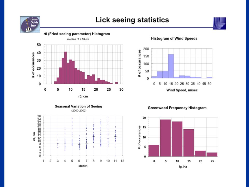
Typical values of r 0 Usually r 0 is given at a 0.5 micron wavelength for reference purposes. It’s up to you to scale it by -1.2 to evaluate r 0 at your favorite wavelength. At excellent sites such as Paranal, r 0 at 0.5 micron is 10 - 30 cm. But there is a big range from night to night, and at times also within a night. r 0 changes its value with a typical time constant of 5-10 minutes

22
Phase PSD, another important parameter Using the Kolmogorov turbulence hypothesis, the atmospheric phase PSD can be derived and is This expression can be used to compute the amount of phase error over an uncorrected pupil

23
Units: Radians of phase / (D / r 0 ) 5/6 Reference: Noll76 Tip-tilt is single biggest contributor Focus, astigmatism, coma also big High-order terms go on and on….
 5/6 Reference: Noll76 Tip-tilt is single biggest contributor Focus, astigmatism, coma also big High-order terms go on and on….")
Similar presentations
 straight lines: the pinhole camera’s inverted image Enlarging the pinhole leads.>")


 and Andrei Tokovinine.>")
 Exit Pupil Entrance Pupil.>")
 2007 1 Figure 3.1 Examples of typical aberrations of construction.>")


