Download presentation
Presentation is loading. Please wait.

1
Regularised Inversion and Model Predictive Uncertainty Analysis

2
PEST …

3
Model Input files Output files

4
Model Input files Output files PEST writes model input files reads model output files

5
Batch or Script File Input files Output files PEST writes model input files reads model output files

6
Model calibration conditions Input files PEST Input files Model predictive conditions Output files

7
Model calibration conditions Input files Model predictive conditions Output files Maximise or minimise key prediction while keeping model calibrated PEST

8
distance or time q1q1 q2q2 q3q3 etc value Model output Field or laboratory measurements and model output:- calibration datasetprediction

9
distance or time q1q1 q2q2 q3q3 etc value Model output Field or laboratory measurements and model output:- calibration dataset Lower predictive limit

10
distance or time q1q1 q2q2 q3q3 etc value Model output Field or laboratory measurements and model output:- calibration dataset Upper predictive limit

11
distance or time q1q1 q2q2 q3q3 etc value Model output Field or laboratory measurements and model output:- calibration dataset Confidence interval for prediction

12
distance or time q1q1 q2q2 q3q3 etc value Model output Field or laboratory measurements and model output:- calibration dataset Predictive uncertainty interval

13
Traditional Parameter Estimation Principal of parsimony Employ no more parameters than can be estimated Calibration complexity dictated by calibration dataset.

14
Regularised inversion…

15
Advantages of Regularised Inversion The inversion process is able to put the heterogeneity exactly where it is needed Maximum information content is extracted from the data Predictive error variance is thus minimised Parameterisation complexity determined by prediction Because complexity is retained in the system, we have the ability to realistic assess predictive uncertainty because we do not exclude the detail on which a prediction can depend.

16
Two Principal Types of Regularisatoin “Tikhonov” – constrained minimisation Subspace methods – principal component analysis

17
SVD-Assist

18
Advantages Highly stable numerically. Highly efficient in model run requirements. Can adapt to noise content of data.

19
Hydraulic conductivity

20
Specific Yield

21
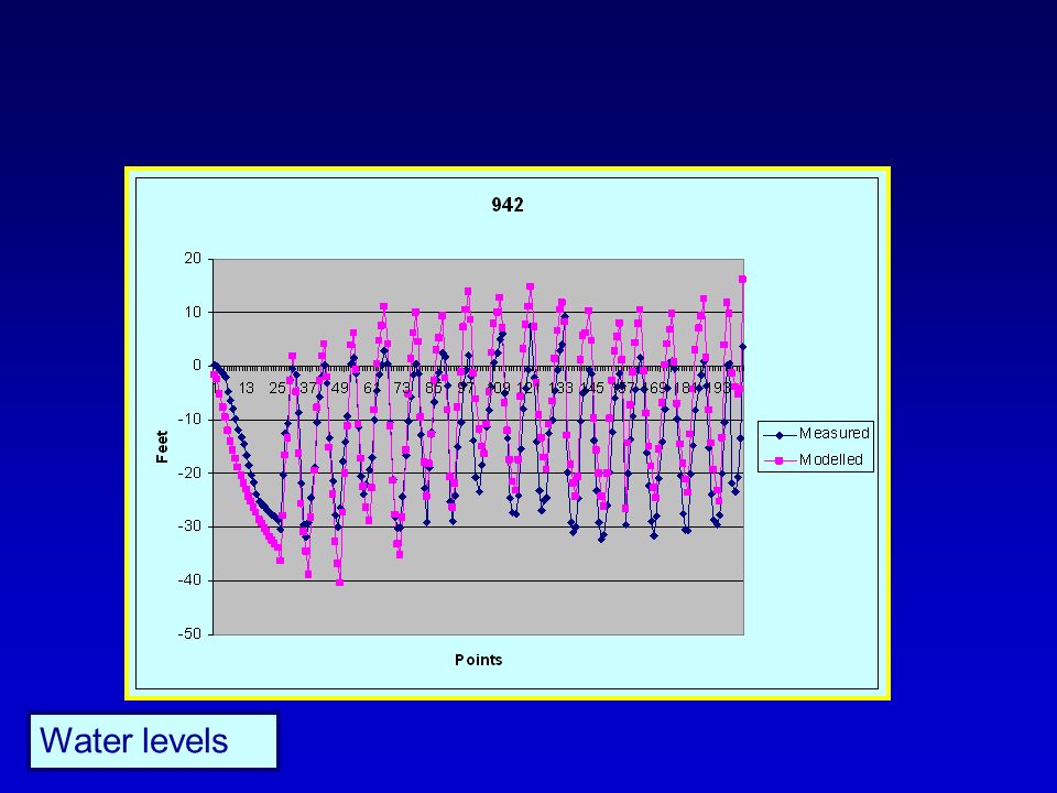
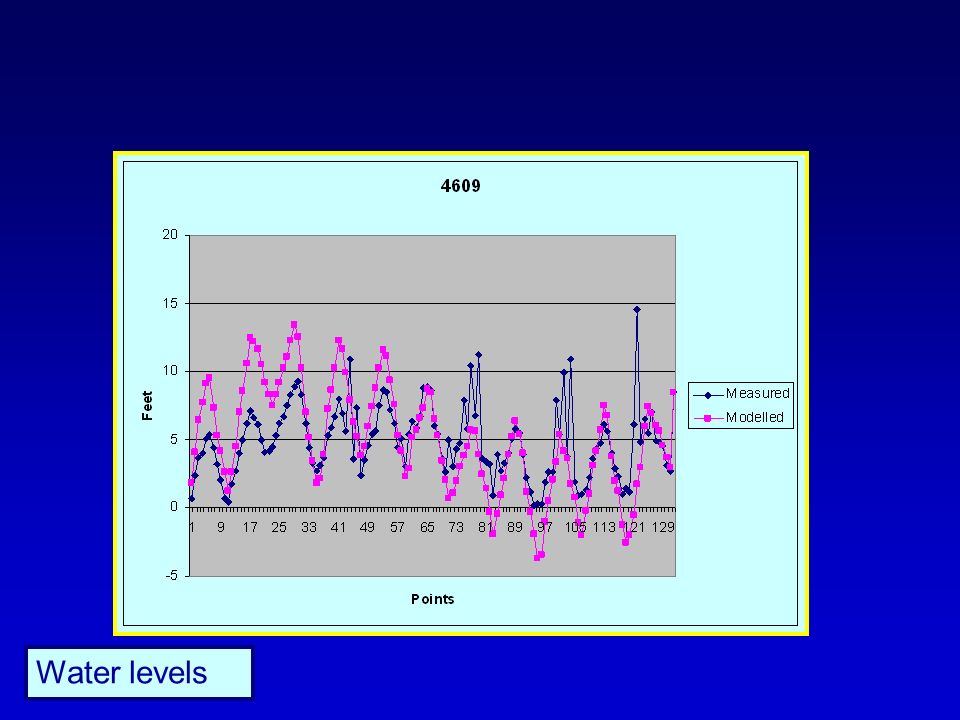
Water levels

25
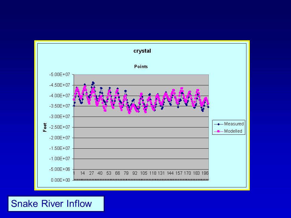
Snake River Inflow

27
Local Domain and Air Photo Recovery Well Source area

28
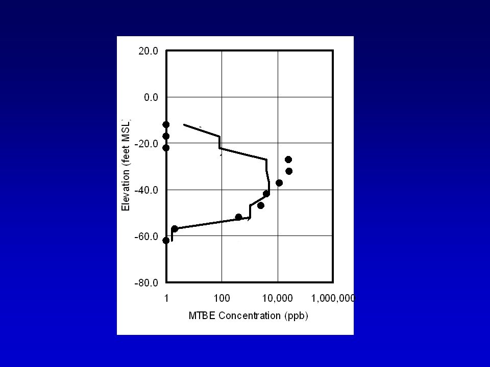
MTBE concentrations for an elevation of:- –35 ft-msl to –40 ft-msl

29
Pilot Points and Observations Pilot points – 58 per layer, L1-L7, for HHK, VHK, POR (crosses). Water level observations (circles); MTBE observations (stars) Calibrated ‘mean’ particle. Recovery Well Source area
; MTBE observations (stars) Calibrated ‘mean’ particle. Recovery Well Source area.")
30
Example Section Profile Profile across plume at IRM transect

31
Figure 4 Typical Concentration Profile

32
Observed MTBE Modelled MTBE -35 to -40 ft msl

37
Profile - data Source Area FLOW

38
Source Area FLOW Profile – data and modelled concentrations

39
Simulated and Observed MTBE at the Recovery Well

40
Calibrated Horizontal and Vertical Hydraulic Conductivities Ground Water Flow

41
The cost of uniqueness …..

42
Model grid Dimensions of model domain 500m by 800m

43
Boundary H = 0.0 Q = 50 m 3 /day

44
Particle release point

45
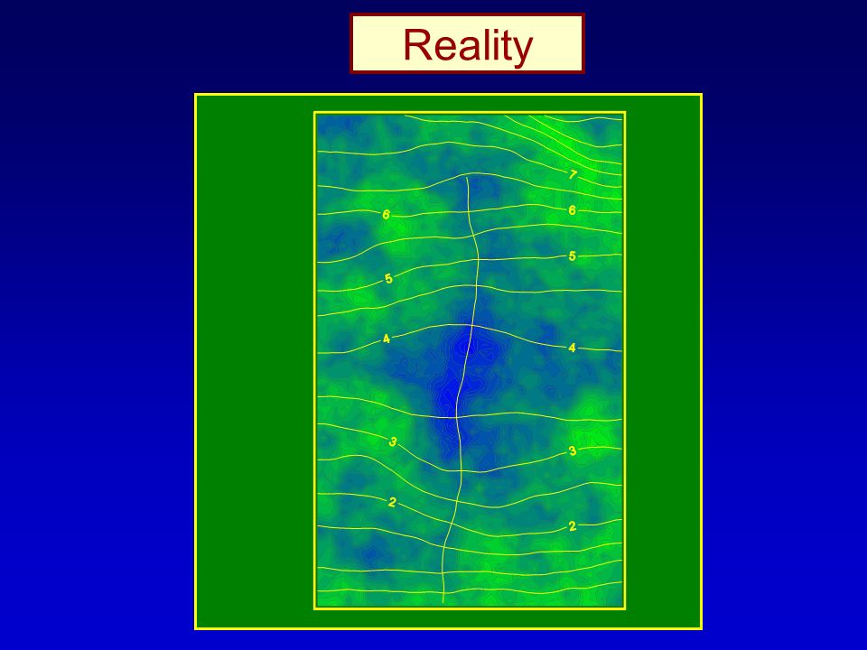
Reality

47
True time = 3256.24 days True exit point = easting of 206.78

48
12 head observations

49
Reality Exit time = 3256 Exit point = 206

50
Calibration to 12 observations (no noise) Exit time = 7122 [true=3256] Exit point = 241 [true=206]
![Calibration to 12 observations (no noise) Exit time = 7122 [true=3256] Exit point = 241 [true=206]](http://images.slideplayer.com/28/9293205/slides/slide_50.jpg "Calibration to 12 observations (no noise) Exit time = 7122 [true=3256] Exit point = 241 [true=206]")
51
This model (with its three parameters)…
…")
52
Calibration to 12 observations Zone-based calibration Exit time = 6364 [true=3256] Exit point = 244 [true=206]
![Calibration to 12 observations Zone-based calibration Exit time = 6364 [true=3256] Exit point = 244 [true=206]](http://images.slideplayer.com/28/9293205/slides/slide_52.jpg "Calibration to 12 observations Zone-based calibration Exit time = 6364 [true=3256] Exit point = 244 [true=206]")
53
… does not even acknowledge the detail upon which a critical prediction will depend, whereas this model ….

54
Calibration to 12 observations (no noise) Exit time = 7122 [true=3256] Exit point = 241 [true=206]
![Calibration to 12 observations (no noise) Exit time = 7122 [true=3256] Exit point = 241 [true=206]](http://images.slideplayer.com/28/9293205/slides/slide_54.jpg "Calibration to 12 observations (no noise) Exit time = 7122 [true=3256] Exit point = 241 [true=206]")
55
Another important point… … does. The former model will grossly under-estimate predictive variance.

56
Calculation of Model Predictive Error Variance…..

57
Parameter space Increasing number of parameter combinations

58
Estimable parameter combinations Unestimable parameter combinations Increasing number of parameter combinations

59
Error variance calculable from measurement error C(h) Error variance supplied by hydrogeologists C(p) Increasing number of parameter combinations
 Error variance supplied by hydrogeologists C(p) Increasing number of parameter combinations")
60
Error variance calculable from measurement error C(h) Error variance supplied by hydrogeologists C(p) model prediction
 Error variance supplied by hydrogeologists C(p) model prediction")
61
σ 2 = y t (I-R) t C(p)(I-R)y + y t GC(h)Gy Therefore total “possible model error” depends on both C(h) and C(p)
 t C(p)(I-R)y + y t GC(h)Gy Therefore total possible model error depends on both C(h) and C(p)")
62
Error variance calculable from measurement error C(h) Error variance supplied by hydrogeologists C(p) model prediction
 Error variance supplied by hydrogeologists C(p) model prediction")
63
Error variance calculable from measurement error C(h) Error variance supplied by hydrogeologists C(p) model prediction Where do we draw the line on what we try to estimate?
 Error variance supplied by hydrogeologists C(p) model prediction Where do we draw the line on what we try to estimate")
64
Number of singular values Predictive error variance “Null space” term “Measurement” term Total Predictive error variance vs dimensions of calibrated parameter space

65
Optimising Data Acquistion…..

66
Schematic block diagram illustrating model layers and boundary conditions

67
The prediction

68
Pumping from layer 3 - 2050

69
Measurements

70
Observation wells Layer 1 Layer 2 Layer 3

71
Water levels

72
Parameters

73
Hydraulic conductivity – layer 1 Hydraulic conductivity – layer 2 Hydraulic conductivity – layer 3 VCONT – layer 2 VCONT – layer 3 Specific yield – layer 1 Specific yield – layer 2 Primary storage capacity – layer 2 Primary storage capacity – layer 3 Riverbed conductance Recharge Parameters included in analysis

74
Pre-calibration contribution to predictive error variance

75
Predictive error variance vs dimensions of calibrated parameter space Minimum = 418 ft 2 at 160 singular values

76
Contribution to pre- and post-calibration predictive variance by selected parameter types

77
Optimization of data acquisition:- How can I deepen the minimum in the predictive variance curve?

78
σ 2 = y t (I-R) t C(p)(I-R)y + y t GC(h)Gy
 t C(p)(I-R)y + y t GC(h)Gy")
79
Reduction in predictive variance if VCONT 2 characterization at each point is reduced from 0.74 to 0.37 (maximum reduction = 112.7ft 2 )
")
80
Locations of proposed layer 2-3 differential head measurements (reduction in predictive error variance = 230 ft 2 )
")
82
Predictive error variance vs dimensions of calibrated parameter space Previous minimum = 418 ft 2 at 160 singular values New minimum = 188 ft 2 at 190 singular values

83
Error variance of an existing model…..

84
IBOUND array

85
Riverbed K parameters

86
Log of K (K ranges from 1e-4 to 500)
")
87
All lateral Inflow Zones (red cells are fixed head – except for zone 1)
")
88
19 2 3 4 56 7 8 9 10 11 12 13 14 15 16 Management zones

89
Head error variance Number of cells

Similar presentations


 Steps in Transport Modeling Calibration step (calibrate flow model & transport model) Adjust parameter values.>")


>")
 Prediction standard deviations (Book, p. 180): A measure of prediction uncertainty Calculated by translating.>")


