Download presentation
Presentation is loading. Please wait.

1
Using HYSPLIT to Understand Source-Receptor Relationships: Some Examples HYSPLIT Training NOAA Air Resources Laboratory Jun 2-4, 2009 Silver Spring, MD, USA Mark Cohen NOAA Air Resources Laboratory 1315 East West Highway, R/ARL, Room 3316 Silver Spring, Maryland, 20910, USA mark.cohen@noaa.gov http://www.arl.noaa.gov/Mercury_modeling.php

2
We use HYSPLIT in many ways at the Air Resources Laboratory to investigate atmospheric source-receptor relationships. A few examples will be shown in this presentation: 1. Back-trajectory analysis of individual measurement “episodes” 2. Back-trajectory “frequency” analysis of measurements

3
We use HYSPLIT in many ways at the Air Resources Laboratory to investigate atmospheric source-receptor relationships. A few examples will be shown in this presentation: 1. Back-trajectory analysis of individual measurement “episodes” 2. Back-trajectory “frequency” analysis of measurements

4
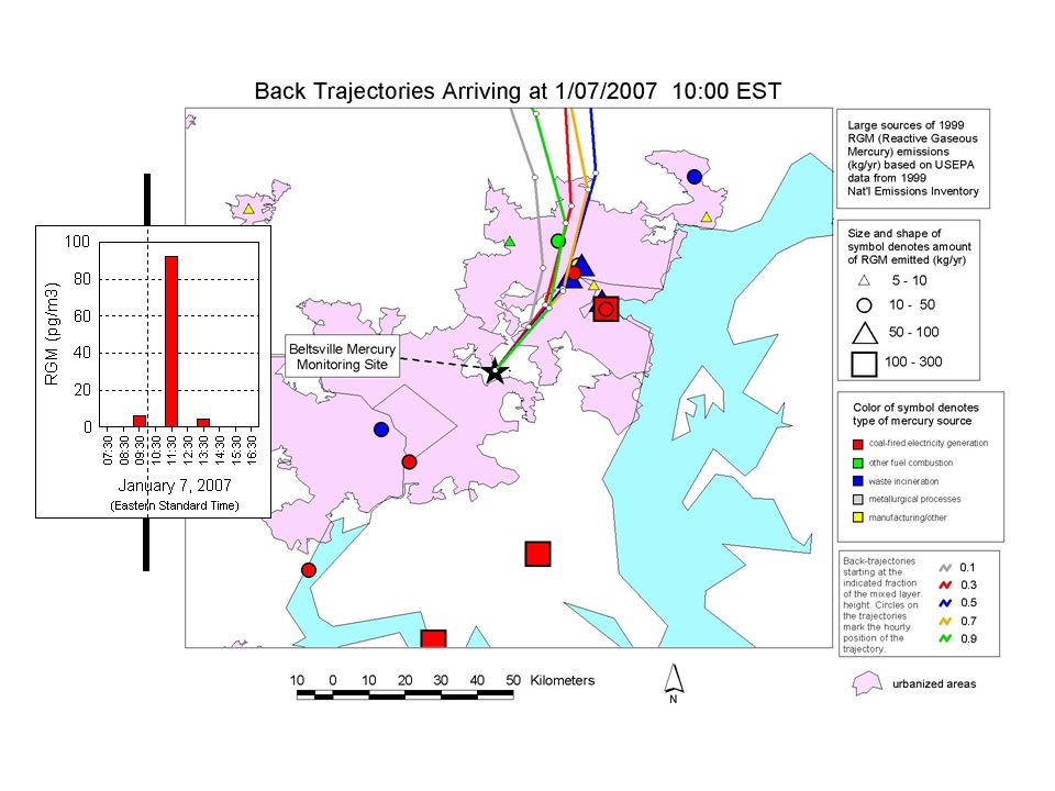
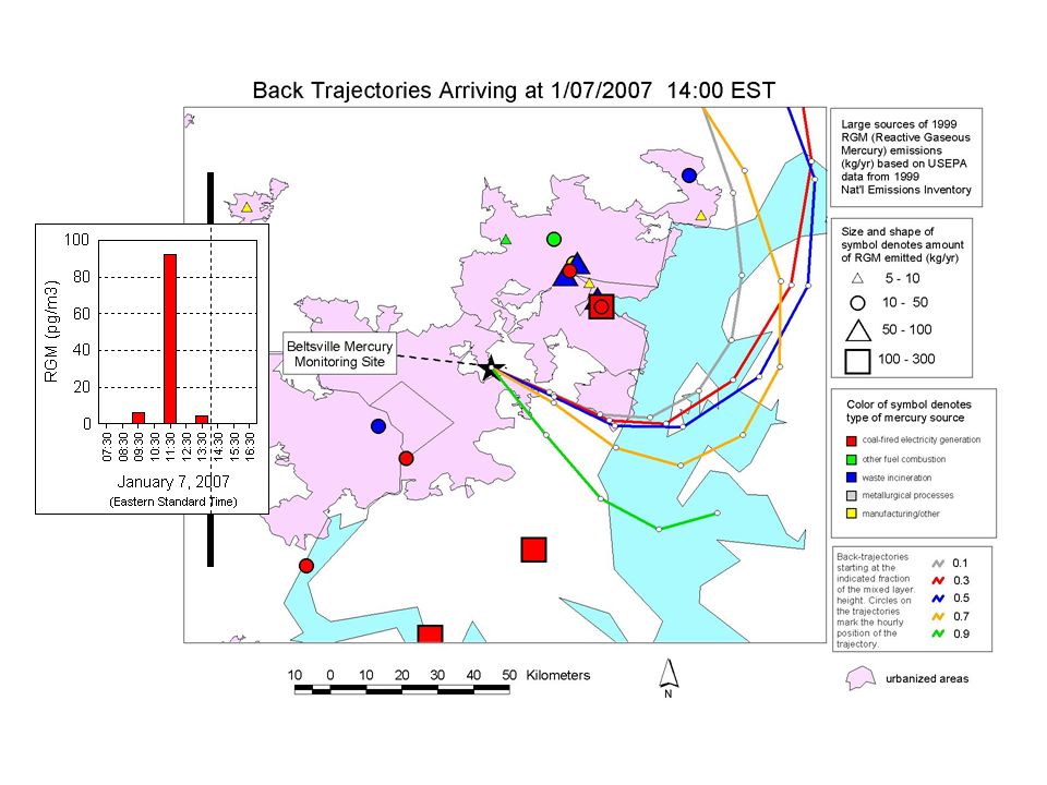
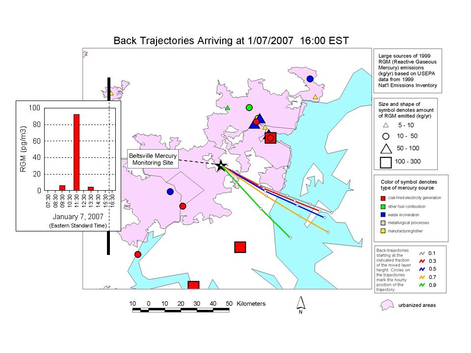
Atmospheric mercury episode at the Beltsville Maryland measurement site on January 7, 2007 Principal Investigator for measurements: Winston Luke, NOAA ARL Beltsville MD mercury site is a collaboration between USEPA, NOAA, others

5
Back trajectories simulated with the NOAA HYSPLIT model using meteorological on a 12 km grid Trajectories started from the Beltsville site (marked with a star on the map) at 5 different heights representing different positions in the mixed layer (0.1, 0.3, 0.5, 0.7, 0.9) Note that the times are represented in UTC (Universal Time Coordinate) which is 5 hours later than Eastern Standard Time, e.g., 17 UTC = 12:00 Eastern Standard Time Large mercury emissions sources are indicated on the map, including: Dick = Dickerson facilities (coal-fired power plant and municipal waste incinerator) Harf = Harford County municipal waste incinerator PhRe = Phoenix Services medical waste and Baltimore Resco municipal waste incinerators BS_W = Brandon Shores and H.A. Wagner coal fired power plants CkPt = Chalk Point coal fired power plant Mrgt = Morgantown coal fired power plant PsPt = Possum Point coal fired power plant Ptmc = Potamac River coal fired power plant Arlg = Arlington/Pentagon waste incinerator Brun = Brunner Island coal fired power plant 100 km

6
display HYSPLIT- generated trajectory shapefiles in GIS program (ArcView) along with emissions
 along with emissions")
17
We use HYSPLIT in many ways at the Air Resources Laboratory to investigate atmospheric source-receptor relationships. A few examples will be shown in this presentation: 1. Back-trajectory analysis of individual measurement “episodes” 2. Back-trajectory “frequency” analysis of measurements

18
Piney Measurement Site Piney Measurement Site and Surrounding Region

19
color of symbol denotes type of mercury source coal-fired power plants other fuel combustion waste incineration metallurgical manufacturing & other size/shape of symbol denotes amount of mercury emitted (kg/yr) 10 - 50 50 - 100 100 – 300 300 - 500 5 - 10 500 - 1000 1000 - 3500 Air Emissions Piney Measurement Site Piney Measurement Site and Surrounding Region with estimated 2002 emissions of total mercury
 – Air Emissions Piney Measurement Site Piney Measurement Site and Surrounding Region with estimated 2002 emissions of total mercury")
20
From Mark Castro, Univ. of Maryland, Frostburg

21
color of symbol denotes type of mercury source coal-fired power plants other fuel combustion waste incineration metallurgical manufacturing & other size/shape of symbol denotes amount of mercury emitted (kg/yr) 10 - 50 50 - 100 100 – 300 300 - 500 5 - 10 500 - 1000 1000 - 3500 Air Emissions Piney Measurement Site EDAS 40km meteorological data grid used for back-trajectory analysis Piney Measurement Site and Surrounding Region with estimated 2002 emissions of total mercury and EDAS 40km meteorological data grid used for back-trajectory analysis
 – Air Emissions Piney Measurement Site EDAS 40km meteorological data grid used for back-trajectory analysis Piney Measurement Site and Surrounding Region with estimated 2002 emissions of total mercury and EDAS 40km meteorological data grid used for back-trajectory analysis")
22
color of symbol denotes type of mercury source coal-fired power plants other fuel combustion waste incineration metallurgical manufacturing & other size/shape of symbol denotes amount of mercury emitted (kg/yr) 10 - 50 50 - 100 100 – 300 300 - 500 5 - 10 500 - 1000 1000 - 3500 Air Emissions Piney Measurement Site EDAS 40km meteorological data grid used for back-trajectory analysis Piney Measurement Site and Surrounding Region with estimated 2002 emissions of total mercury and EDAS 40km meteorological data grid used for back-trajectory analysis
 – Air Emissions Piney Measurement Site EDAS 40km meteorological data grid used for back-trajectory analysis Piney Measurement Site and Surrounding Region with estimated 2002 emissions of total mercury and EDAS 40km meteorological data grid used for back-trajectory analysis")
23
The mercury monitor is about 5 meters above the ground and the actual elevation of site is 769 m above sea level But the EDAS 40km meteorological data “Terrain Height” for this location is about 600 m What starting height should be used for back-trajectories? In this study we used a starting height of ½ of the Planetary Boundary Layer (PBL) as represented in the meteorological data set In this study we used a starting height of ½ of the Planetary Boundary Layer (PBL) as represented in the meteorological data set
 as represented in the meteorological data set In this study we used a starting height of ½ of the Planetary Boundary Layer (PBL) as represented in the meteorological data set.")
24
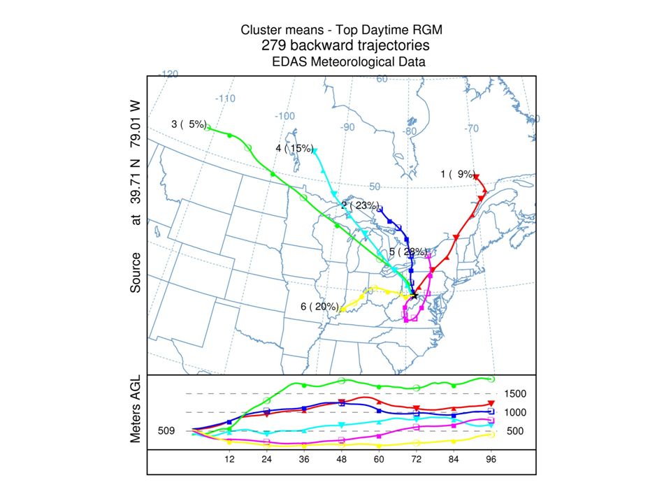
Top Daytime RGM Up to 6 clusters, we see an improvement, With more than 6 clusters, little improvement So, 6 clusters may be optimal

26
Cluster means – Top Daytime RGM (regional view) 20% 28% 5% 15% 9% 23% color of symbol denotes type of mercury source coal-fired power plants other fuel combustion waste incineration metallurgical manufacturing & other size/shape of symbol denotes amount of mercury emitted (kg/yr) 10 - 50 50 - 100 100 – 300 300 - 500 5 - 10 500 - 1000 1000 - 3500 Air Emissions Piney Measurement Site
 20% 28% 5% 15% 9% 23% color of symbol denotes type of mercury source coal-fired power plants other fuel combustion waste incineration metallurgical manufacturing & other size/shape of symbol denotes amount of mercury emitted (kg/yr) – Air Emissions Piney Measurement Site")
27
Trajectory Endpoint Frequency Graphics 0.5 degree lat/long grid Starting height for all trajectories in this group = ½ planetary boundary layer height Decided to try a different approach --

28
Spatial distribution of hourly trajectory endpoint frequencies Entire year, Starting Height = ½ Planetary Boundary Layer color of symbol denotes type of mercury source coal-fired power plants other fuel combustion waste incineration metallurgical manufacturing & other size/shape of symbol denotes amount of mercury emitted (kg/yr) 10 - 50 50 - 100 100 – 300 300 - 500 5 - 10 500 - 1000 1000 - 3500 Percent of back-trajectories passing through grid square 0 - 1 1- 5 5 - 10 10 - 25 25 - 100 Air Emissions Piney Measurement Site with estimated 2002 emissions of reactive gaseous mercury 0.5 degree lat/long grid
 – Percent of back-trajectories passing through grid square Air Emissions Piney Measurement Site with estimated 2002 emissions of reactive gaseous mercury 0.5 degree lat/long grid")
29
Spatial distribution of hourly trajectory endpoint frequencies color of symbol denotes type of mercury source coal-fired power plants other fuel combustion waste incineration metallurgical manufacturing & other size/shape of symbol denotes amount of mercury emitted (kg/yr) 10 - 50 50 - 100 100 – 300 300 - 500 5 - 10 500 - 1000 1000 - 3500 Percent of back-trajectories passing through grid square 0 - 1 1- 5 5 - 10 10 - 25 25 - 100 Air Emissions Piney Measurement Site RGM Top 10% (day 8 AM – 6 PM) Starting Height = ½ Planetary Boundary Layer with estimated 2002 emissions of reactive gaseous mercury 0.5 degree lat/long grid
 – Percent of back-trajectories passing through grid square Air Emissions Piney Measurement Site RGM Top 10% (day 8 AM – 6 PM) Starting Height = ½ Planetary Boundary Layer with estimated 2002 emissions of reactive gaseous mercury 0.5 degree lat/long grid")
30
Spatial distribution of hourly trajectory endpoint frequencies color of symbol denotes type of mercury source coal-fired power plants other fuel combustion waste incineration metallurgical manufacturing & other size/shape of symbol denotes amount of mercury emitted (kg/yr) 10 - 50 50 - 100 100 – 300 300 - 500 5 - 10 500 - 1000 1000 - 3500 Percent of back-trajectories passing through grid square 0 - 1 1- 5 5 - 10 10 - 25 25 - 100 Air Emissions Piney Measurement Site RGM Bottom 10% (day 8 AM – 6 PM) Starting Height = ½ Planetary Boundary Layer with estimated 2002 emissions of reactive gaseous mercury 0.5 degree lat/long grid
 – Percent of back-trajectories passing through grid square Air Emissions Piney Measurement Site RGM Bottom 10% (day 8 AM – 6 PM) Starting Height = ½ Planetary Boundary Layer with estimated 2002 emissions of reactive gaseous mercury 0.5 degree lat/long grid")
31
Trajectory Endpoint Frequency Graphics 0.1 degree lat/long regional grid Starting height for all trajectories in this group = ½ planetary boundary layer height Same analysis, but now with 0.1 degree grid…

32
Spatial distribution of hourly trajectory endpoint frequencies Entire year, Starting Height = ½ Planetary Boundary Layer color of symbol denotes type of mercury source coal-fired power plants other fuel combustion waste incineration metallurgical manufacturing & other size/shape of symbol denotes amount of mercury emitted (kg/yr) 10 - 50 50 - 100 100 – 300 300 - 500 5 - 10 500 - 1000 1000 - 3500 Percent of back-trajectories passing through grid square 0 - 1 1- 3 3 - 6 6 – 10 10 - 100 Air Emissions Piney Measurement Site with estimated 2002 emissions of reactive gaseous mercury 0.1 degree lat/long regional grid
 – Percent of back-trajectories passing through grid square – Air Emissions Piney Measurement Site with estimated 2002 emissions of reactive gaseous mercury 0.1 degree lat/long regional grid")
33
Cluster means – Top Daytime RGM (regional view) 20% 28% 5% 15% 9% 23% color of symbol denotes type of mercury source coal-fired power plants other fuel combustion waste incineration metallurgical manufacturing & other size/shape of symbol denotes amount of mercury emitted (kg/yr) 10 - 50 50 - 100 100 – 300 300 - 500 5 - 10 500 - 1000 1000 - 3500 Air Emissions Piney Measurement Site
 20% 28% 5% 15% 9% 23% color of symbol denotes type of mercury source coal-fired power plants other fuel combustion waste incineration metallurgical manufacturing & other size/shape of symbol denotes amount of mercury emitted (kg/yr) – Air Emissions Piney Measurement Site")
34
Spatial distribution of hourly trajectory endpoint frequencies RGM Top 10% (day 8 AM – 6 PM) Starting Height = ½ Planetary Boundary Layer with estimated 2002 emissions of reactive gaseous mercury color of symbol denotes type of mercury source coal-fired power plants other fuel combustion waste incineration metallurgical manufacturing & other size/shape of symbol denotes amount of mercury emitted (kg/yr) 10 - 50 50 - 100 100 – 300 300 - 500 5 - 10 500 - 1000 1000 - 3500 Percent of back-trajectories passing through grid square 0 - 1 1- 3 3 - 6 6 – 10 10 - 100 Air Emissions Piney Measurement Site 0.1 degree lat/long regional grid
 Starting Height = ½ Planetary Boundary Layer with estimated 2002 emissions of reactive gaseous mercury color of symbol denotes type of mercury source coal-fired power plants other fuel combustion waste incineration metallurgical manufacturing & other size/shape of symbol denotes amount of mercury emitted (kg/yr) – Percent of back-trajectories passing through grid square – Air Emissions Piney Measurement Site 0.1 degree lat/long regional grid")
35
Spatial distribution of hourly trajectory endpoint frequencies RGM Bottom 10% (day 8 AM – 6 PM) Starting Height = ½ Planetary Boundary Layer with estimated 2002 emissions of reactive gaseous mercury color of symbol denotes type of mercury source coal-fired power plants other fuel combustion waste incineration metallurgical manufacturing & other size/shape of symbol denotes amount of mercury emitted (kg/yr) 10 - 50 50 - 100 100 – 300 300 - 500 5 - 10 500 - 1000 1000 - 3500 Percent of back-trajectories passing through grid square 0 - 1 1- 3 3 - 6 6 – 10 10 - 100 Air Emissions Piney Measurement Site 0.1 degree lat/long regional grid
 Starting Height = ½ Planetary Boundary Layer with estimated 2002 emissions of reactive gaseous mercury color of symbol denotes type of mercury source coal-fired power plants other fuel combustion waste incineration metallurgical manufacturing & other size/shape of symbol denotes amount of mercury emitted (kg/yr) – Percent of back-trajectories passing through grid square – Air Emissions Piney Measurement Site 0.1 degree lat/long regional grid")
36
Trajectory Endpoint Frequency Graphics showing the difference in grid frequencies between the trajectories corresponding to a given set of measurements and those for the entire year 0.5 degree lat/long regional grid Starting height for all trajectories in this group = ½ planetary boundary layer height Back to 0.5 degree grid, but now look at differences…

37
Spatial distribution of hourly trajectory endpoint frequencies top 10% of daytime RGM vs. total year color of symbol denotes type of mercury source coal-fired power plants other fuel combustion waste incineration metallurgical manufacturing & other size/shape of symbol denotes amount of mercury emitted (kg/yr) 10 - 50 50 - 100 100 – 300 300 - 500 5 - 10 500 - 1000 1000 - 3500 Difference between two cases in percent of back- trajectories passing through grid square -13 to -4 -4 to -1 -1 to 1 1 to 4 4 to 7 Air Emissions Piney Measurement Site with estimated 2002 emissions of reactive gaseous mercury 0.5 degree lat/long regional grid 7 to 22 The yellow and orange grid squares are areas where the trajectories pass more often than the “average” for the entire year The purple grid squares represent areas where the trajectories pass less often than the “average” for the entire year
 – Difference between two cases in percent of back- trajectories passing through grid square -13 to to to 1 1 to 4 4 to 7 Air Emissions Piney Measurement Site with estimated 2002 emissions of reactive gaseous mercury 0.5 degree lat/long regional grid 7 to 22 The yellow and orange grid squares are areas where the trajectories pass more often than the average for the entire year The purple grid squares represent areas where the trajectories pass less often than the average for the entire year.")
38
Spatial distribution of hourly trajectory endpoint frequencies bottom 10% of daytime RGM vs. total year color of symbol denotes type of mercury source coal-fired power plants other fuel combustion waste incineration metallurgical manufacturing & other size/shape of symbol denotes amount of mercury emitted (kg/yr) 10 - 50 50 - 100 100 – 300 300 - 500 5 - 10 500 - 1000 1000 - 3500 Difference between two cases in percent of back- trajectories passing through grid square -13 to -4 -4 to -1 -1 to 1 1 to 4 4 to 7 Air Emissions Piney Measurement Site with estimated 2002 emissions of reactive gaseous mercury 0.5 degree lat/long regional grid 7 to 22 The yellow and orange grid squares are areas where the trajectories pass more often than the “average” for the entire year The purple grid squares represent areas where the trajectories pass less often than the “average” for the entire year
 – Difference between two cases in percent of back- trajectories passing through grid square -13 to to to 1 1 to 4 4 to 7 Air Emissions Piney Measurement Site with estimated 2002 emissions of reactive gaseous mercury 0.5 degree lat/long regional grid 7 to 22 The yellow and orange grid squares are areas where the trajectories pass more often than the average for the entire year The purple grid squares represent areas where the trajectories pass less often than the average for the entire year.")
39
Trajectory Endpoint Frequency Graphics showing the difference in grid frequencies between the trajectories corresponding to a given set of measurements and those for the entire year 0.1 degree lat/long regional grid Starting height for all trajectories in this group = ½ planetary boundary layer height Finally, differences with 0.1 degree grid…

40
Spatial distribution of hourly trajectory endpoint frequencies top 10% of daytime RGM vs. total year with estimated 2002 emissions of reactive gaseous mercury 0.1 degree lat/long regional grid color of symbol denotes type of mercury source coal-fired power plants other fuel combustion waste incineration metallurgical manufacturing & other size/shape of symbol denotes amount of mercury emitted (kg/yr) 10 - 50 50 - 100 100 – 300 300 - 500 5 - 10 500 - 1000 1000 - 3500 Difference between selected case and total year in percent of back-trajectories passing through grid square < -2.5 -2.5 to -2 -2 to -1.5 Air Emissions Piney Measurement Site -1.5 to -1 -1 to -0.5 -0.5 to 0 > 2.5 2 – 2.5 1.5 - 2 1 to 1.5 0.5 - 1 0 to 0.5 The yellow and orange grid squares are areas where the trajectories pass more often than the “average” for the entire year The purple grid squares represent areas where the trajectories pass less often than the “average” for the entire year
 – Difference between selected case and total year in percent of back-trajectories passing through grid square < to to -1.5 Air Emissions Piney Measurement Site -1.5 to to to 0 > – to to 0.5 The yellow and orange grid squares are areas where the trajectories pass more often than the average for the entire year The purple grid squares represent areas where the trajectories pass less often than the average for the entire year.")
41
Spatial distribution of hourly trajectory endpoint frequencies bottom 10% of daytime RGM vs. total year with estimated 2002 emissions of reactive gaseous mercury 0.1 degree lat/long regional grid color of symbol denotes type of mercury source coal-fired power plants other fuel combustion waste incineration metallurgical manufacturing & other size/shape of symbol denotes amount of mercury emitted (kg/yr) 10 - 50 50 - 100 100 – 300 300 - 500 5 - 10 500 - 1000 1000 - 3500 Difference between selected case and total year in percent of back-trajectories passing through grid square < -2.5 -2.5 to -2 -2 to -1.5 Air Emissions Piney Measurement Site -1.5 to -1 -1 to -0.5 -0.5 to 0 > 2.5 2 – 2.5 1.5 - 2 1 to 1.5 0.5 - 1 0 to 0.5 The yellow and orange grid squares are areas where the trajectories pass more often than the “average” for the entire year The purple grid squares represent areas where the trajectories pass less often than the “average” for the entire year
 – Difference between selected case and total year in percent of back-trajectories passing through grid square < to to -1.5 Air Emissions Piney Measurement Site -1.5 to to to 0 > – to to 0.5 The yellow and orange grid squares are areas where the trajectories pass more often than the average for the entire year The purple grid squares represent areas where the trajectories pass less often than the average for the entire year.")
42
Thanks!

Similar presentations


>")


 College Park, MD, USA Meeting with John Sherwell, Power Plant Research.>")


>")
