1. Chapter 5 無機物理方法（核磁共振部分）
The Physical Methods in Inorganic Chemistry (Fall Term, 2004) (Fall Term, 2005) Department of Chemistry National Sun Yat-sen University
Chapter 5

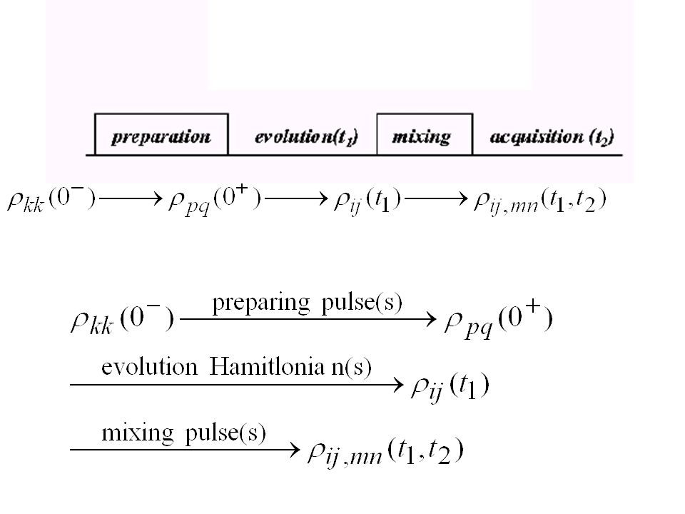
2. Basic Two-Dimensional Experiments
Why multi-dimensional?
Resolution
Multi-quantum coherences
Coherence transfer
Types of multi-dimensional spectra:
To Correlate
To Resolve
To Exchange (Diffusion)

3. From 1D to 2D, 3D… t2 t1

4. If you look at the same data matrix in a different way….
You also get a series of FIDs.

5. In either direction, you see FIDs
You really don’t know which is “acquisition
dimension”, Do you?

6. F2
A 2D Spectrum t2
FT2
FT1 F1 t1

7. 2D FT

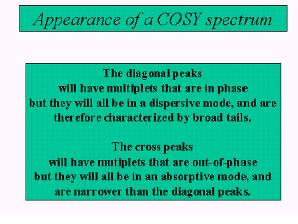
9. Typical 2D Lineshapes

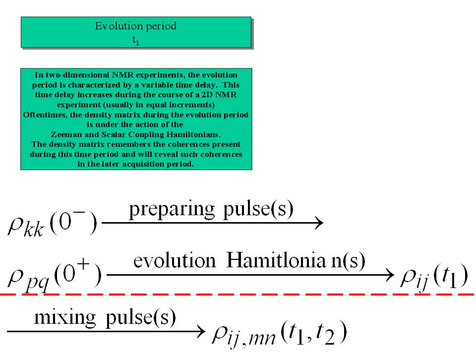
10. Resolution
The resolution in the second dimension is determined the same way
as in 1D NMR.
The resolution in the first dimension is determined by the longest evolution
time in the first dimension (maximum of t1).
The total evolution time in the indirect dimension is equivalent to the total
acquisition time in the detection dimension.

14. Acquisition and data processing:F2 F1

16. COSY pulse sequence (top) with a presaturation pulse to suppress
water signal. Also shown in the diagram are the coherence transfer
pathway (middle) and phase cycling scheme (bottom).

19. COSY pulse sequence (top) with a presaturation pulse to suppress
water signal. Also shown in the diagram are the coherence transfer
pathway (middle) and phase cycling scheme (bottom).

23. Recollecting Chapter 2

24. Four basic lineshapes Anti-phase absorptive FT Real part
In-phase dispersive
FT Real part
Anti-phase dispersive
FT Real part
FT Real part
In-phase absorptive

25. A 2D dispersive peak

26. A 2D absorptive peak

28. + -

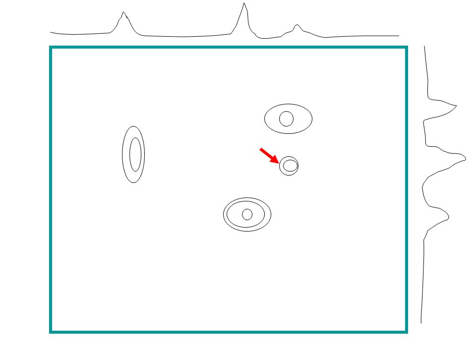
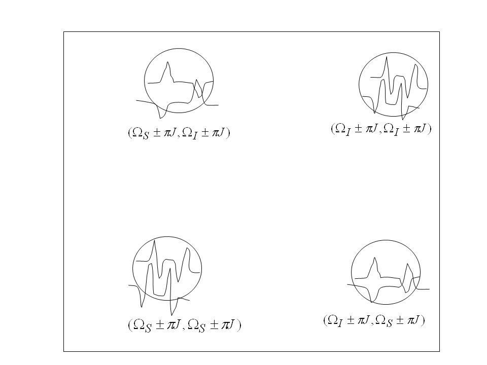
30. Absorptive cross peaks
Dispersive diagonal peaks
Dispersive cross peaks
Absorptive diagonal peaks

31. Absorptive cross peaks

32. Absorptive cross peaks

33. Dispersive diagonal peaks

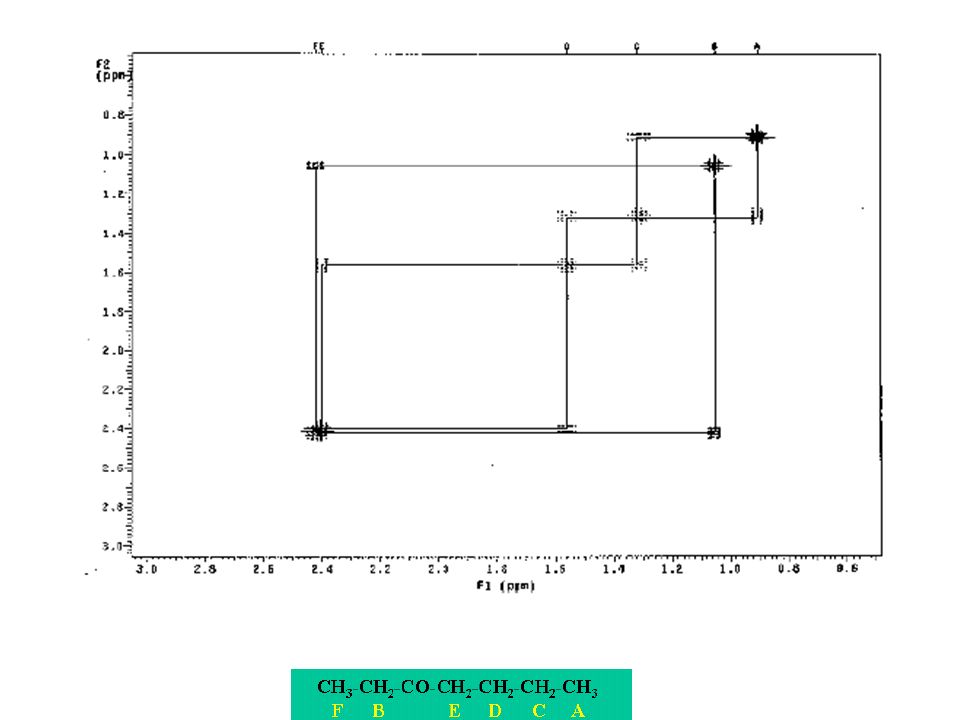
34. F E D C B A

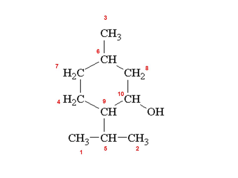
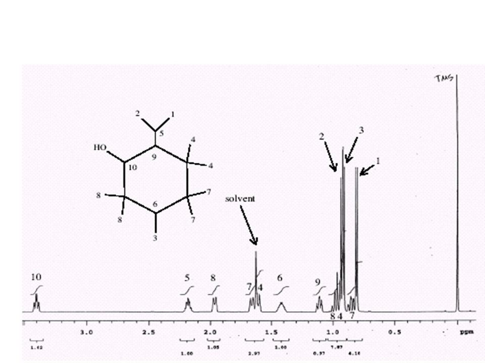
36. 1 2 5 3 4 6 7 8 9 10

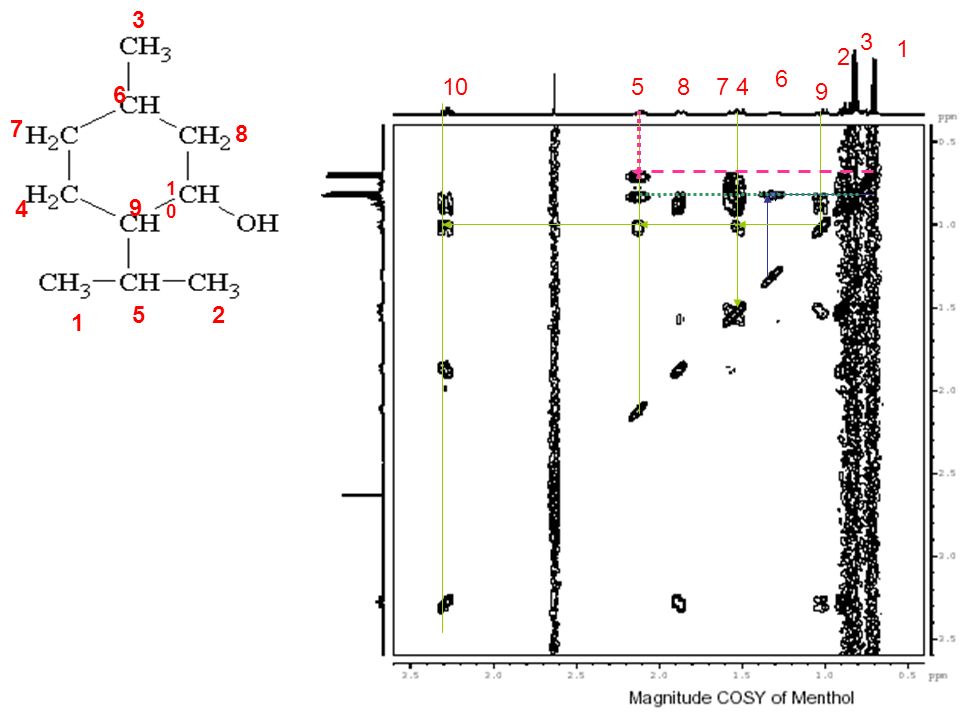
37. 1 2 5 3 4 6 7 8 9 10 1 3 2 9 6
7 4 8 5 10

38. Absolute Value Display

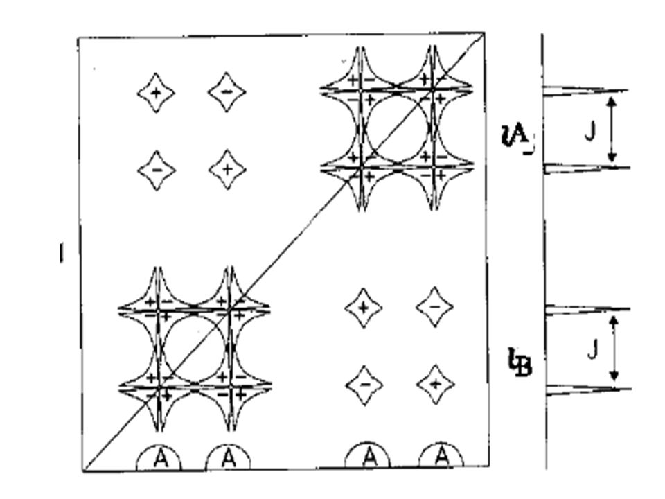
39. The major drawback of COSY: cross peaks
near the diagonal line may be obscured by
diagonal peaks.

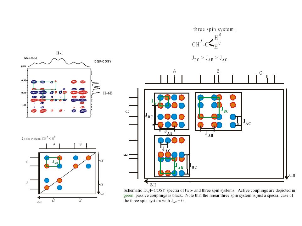
42. DQF COSY

43. 1 2 5 3 4 6 7 8 9 10

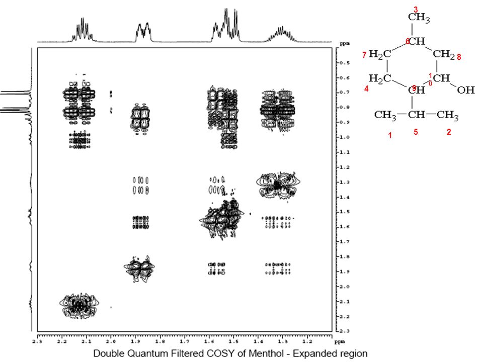
44. 1 2 5 3 4 6 7 8 9 10

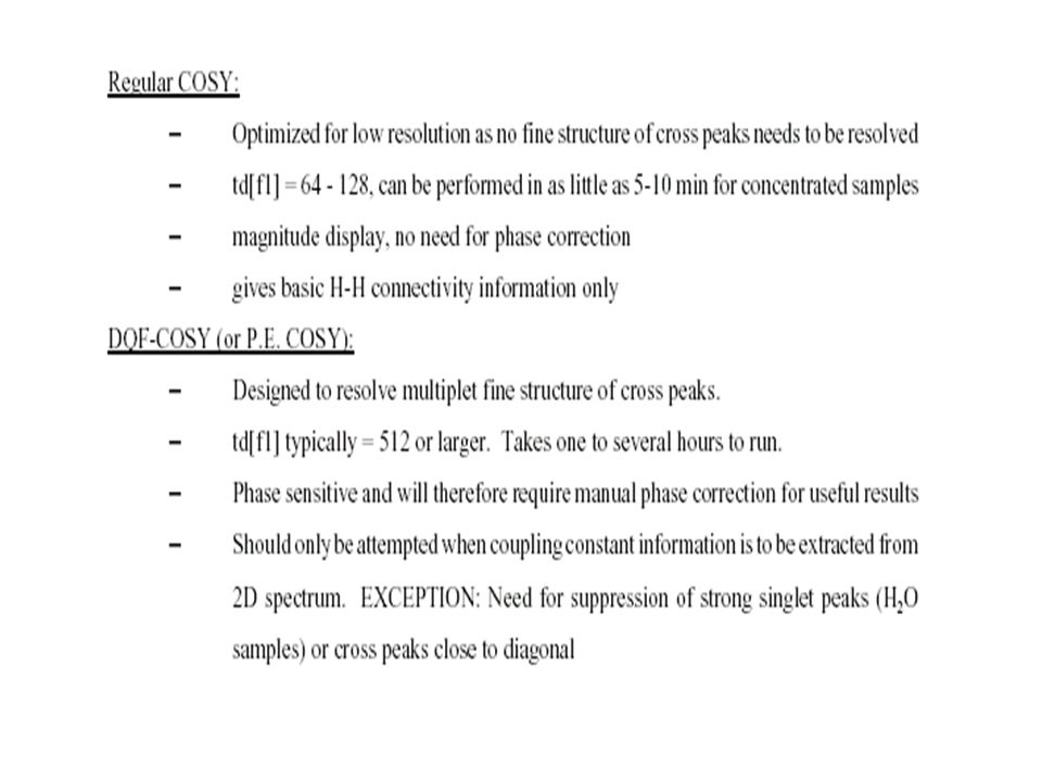
47. The Advantages of DQF COSY
Having the same phase for both the diagonal and cross peaks;
Because the magnetization is detected in anti-phase, the multiplet structure is
retained with opposite phase. In other words, the two lines of a doublet are 180° out
of phase with respect to each other. While this can lead to cancellation in crowded
regions of the spectrum, it also allows for the easy identification of multiplets
(based on their square, or box, shape), and for measuring the size of the scalar
coupling constant connecting the two spins.
Another advantage of the DQF-COSY experiment is not so immediately obvious. In order
for a transition to create multiple quantum levels, and to survive a multiple quantum filter,
you need to have at least two spins or three spins for a 2Q or 3Q transition, respectively.
Thus, singlets are drastically reduced in intensity in a DQF-COSY spectrum.

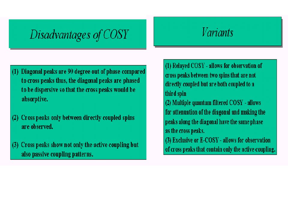
48. The Disadvantages of DQF COSY
There are also disadvantages to the DQF-COSY relative to COSY. First, the sensitivity of DQF is about a factor of two lower than regular COSY. Second, MQ relaxation in 1Hs is very slow, so the experiments require a relatively long d1 relaxation delay.
Thus, while a good COSY spectrum could be generated in about 2-4 hours of data accumulation, a good DQF-COSY requires about hours to allow complete relaxation during d1.

51. ε δ γ β α

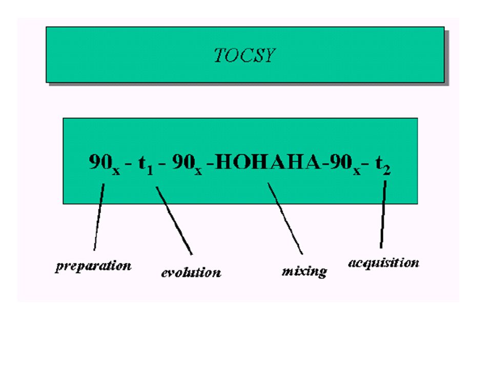
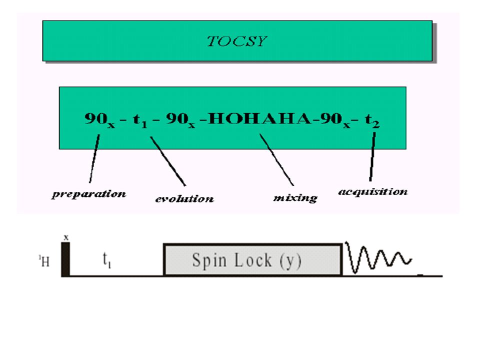
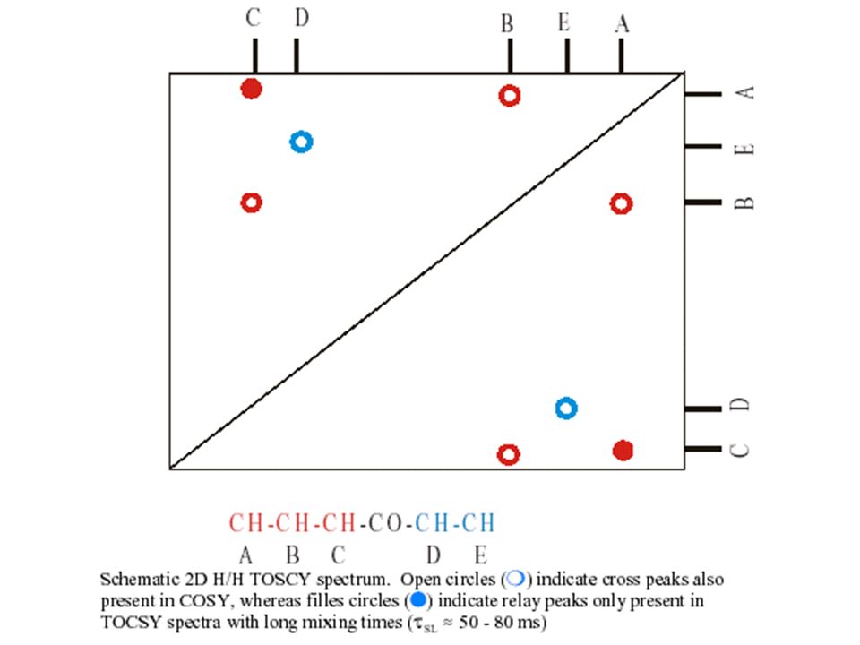
52. TOCSY region of amide protons from residues Lysine 29 and 48

53. TOCSY of BPTI
at different pressures

54. TOCSY of BPTI
at different pressures

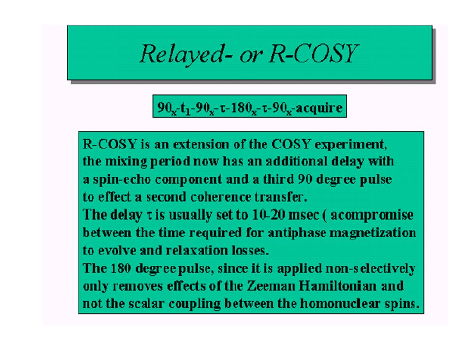
55. COSY Family COSY COSY-45,COSY-90 R-COSY (LR-COSY) pQF COSY PE-COSY
MQ COSY
TOCSY
zCOSY,zzCOSY, J.R.COSY
…..

56. 3JHNα = 5.9 cos2Φ - 1.3cos Φ
3Jαβ = 9.5 cos2χ cosχ1+ 1.8

57. J Coupling Measurement
J coupling and peak intensity
J coupling and linewidth
J coupling and overlap

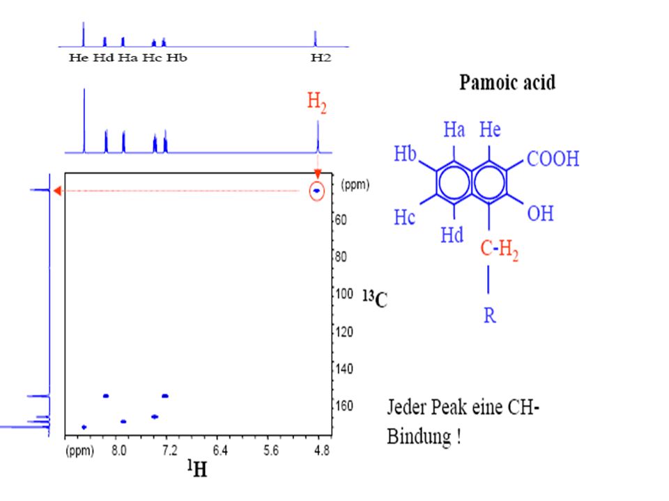
58. Basic Heteronuclear 2D Experiments
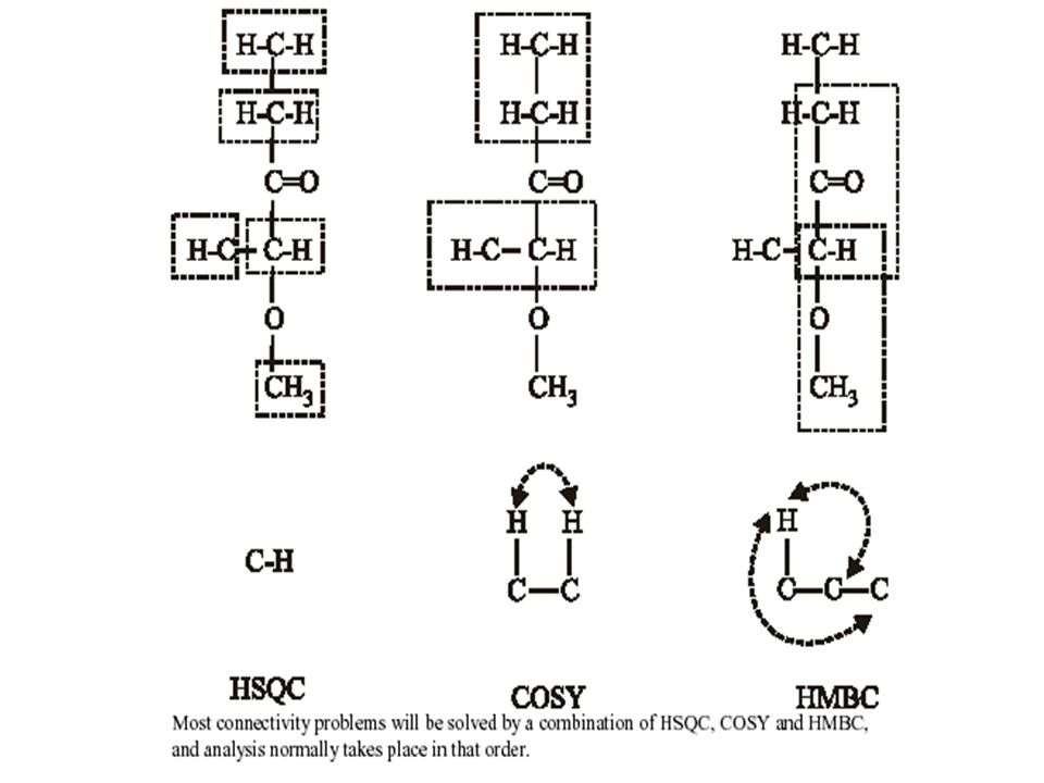
Introduction
Heteronuclear correlation (HETCOR) and its variants (COLOC, HMBC etc)
Heteronuclear multiple-quantum coherence (HMQC)
Heteronuclear single-quantum coherence (HSQC)

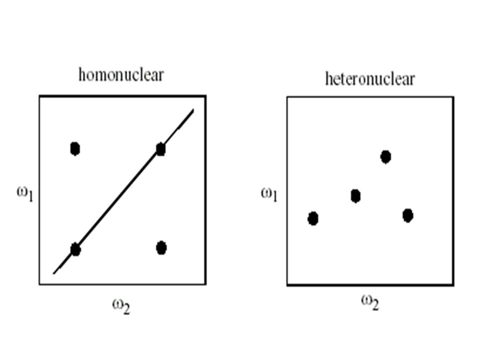
59. Introduction
The availability of other (“hetero”) nuclei than proton for multi-dimensional NMR spectroscopy is extremely useful, particularly, for macromolecules (of synthetic or biological origin) because the connectivity between protons and heteronuclear spins can be established in addition to the homonuclear multi-dimensional spectra.
Like homonuclear 2D spectroscopy, the central task in heteronulcear 2D experiments is to select proper coherence pathways so that the desired interaction can be elucidated. Heteronuclear 2D experiments can be more diverse because, e.g., the data acquisition can be carried out on heteronuclei (C-13, N-15 etc) or on protons (inverse detection).

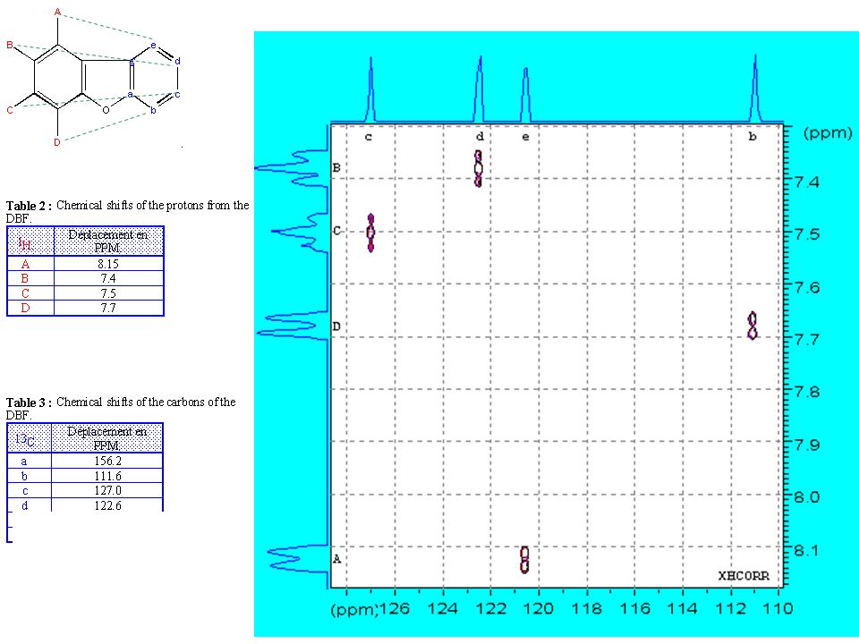
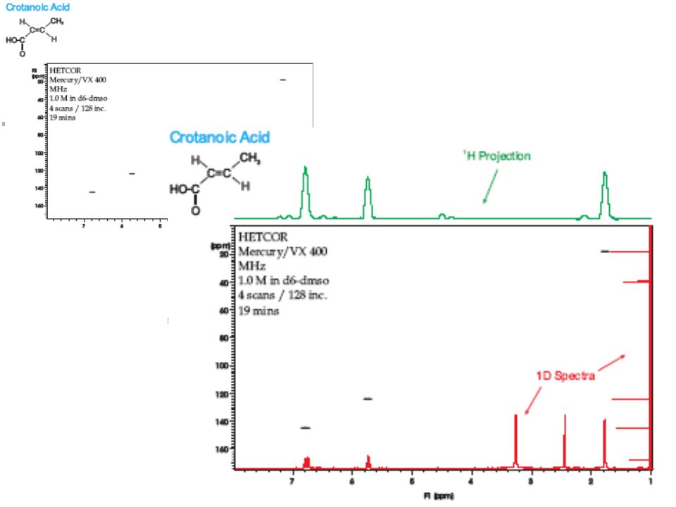
62. Heteronuclear correlation (HETCOR) and its variants

63. During t1, the carbons that are coupled to protons are selected so that only those carbons are “visible” in the detection period. The choice of two fixed delays Δ1 and Δ2 is determined by smallest J-coupling we want to observe, i.e., when long- range coupled carbons (in addition to directly bonded carbons) are also to be observed: Δ1=1/2Jmin, Δ2=1/3Jmin.

64. Enhanced Heteronuclear Correlation
S(δI, δS) ωI ωS

67. COrrelation via LOng-range Coupling(COLOC)
The choice of two fixed delays Δ1 and Δ2 is determined by
smallest J-coupling we want to observe, i.e., when long- range
coupled carbons (in addition to directly bonded carbons) are
also to be observed: Δ1=1/2Jmin, Δ2=1/3Jmin.

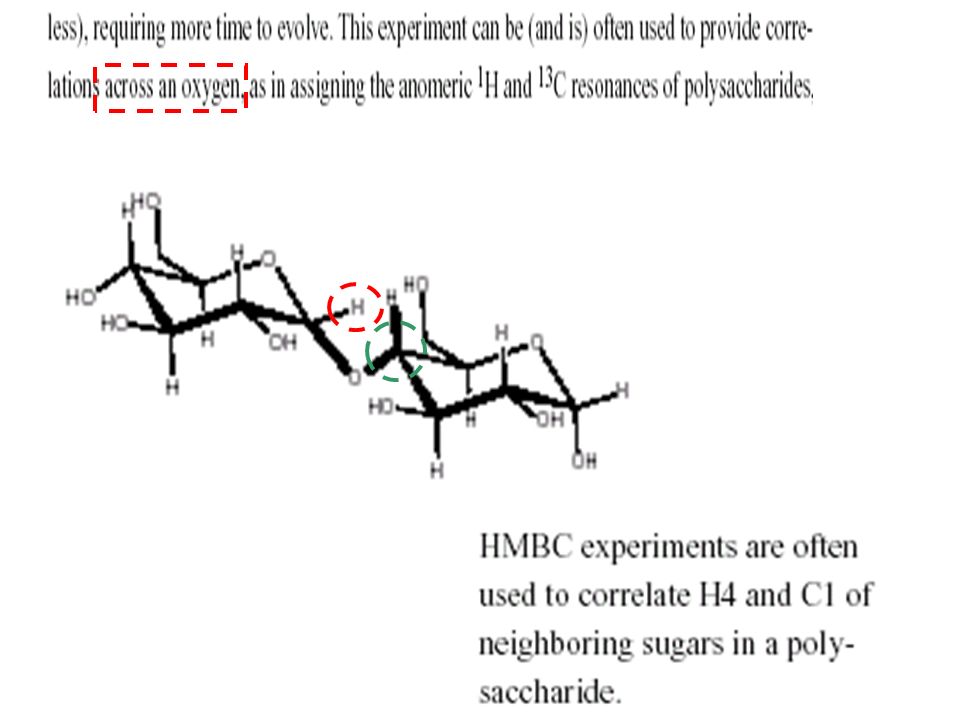
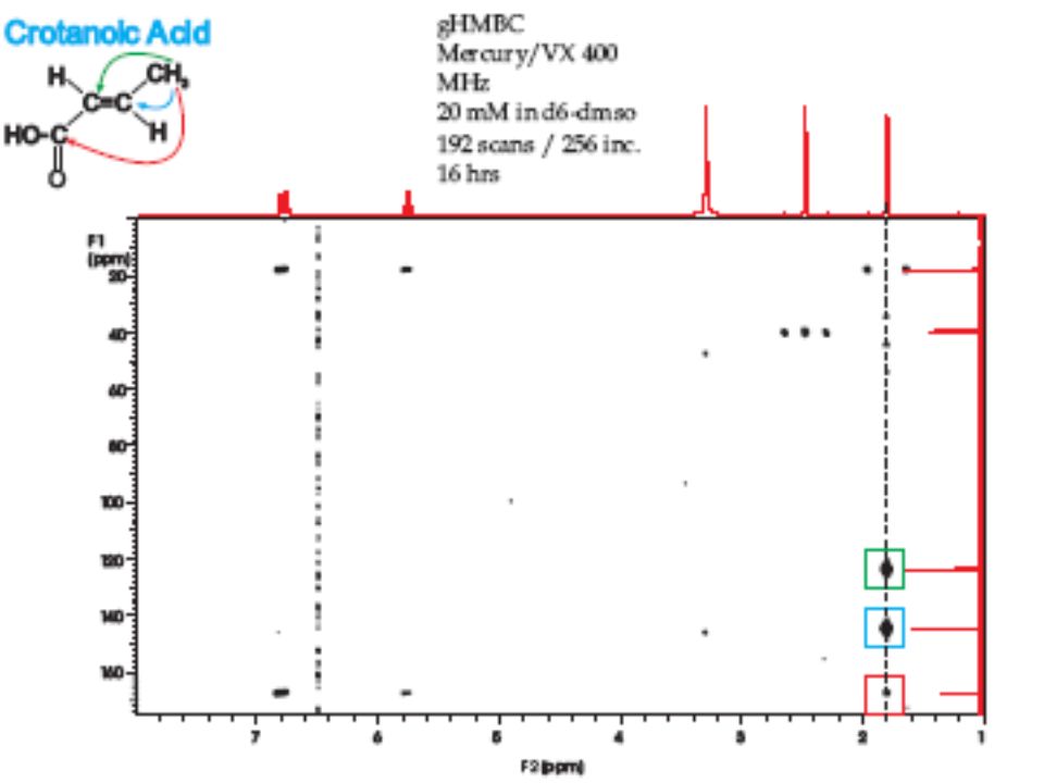
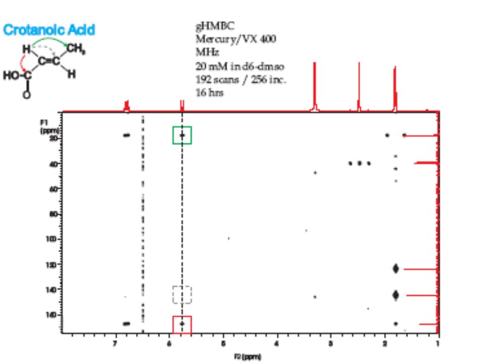
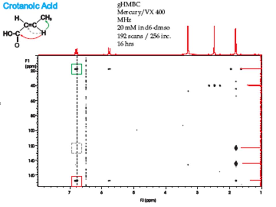
69. Heteronuclear Multi-Bond Correlation (HMBC)

74. Inverse Detection

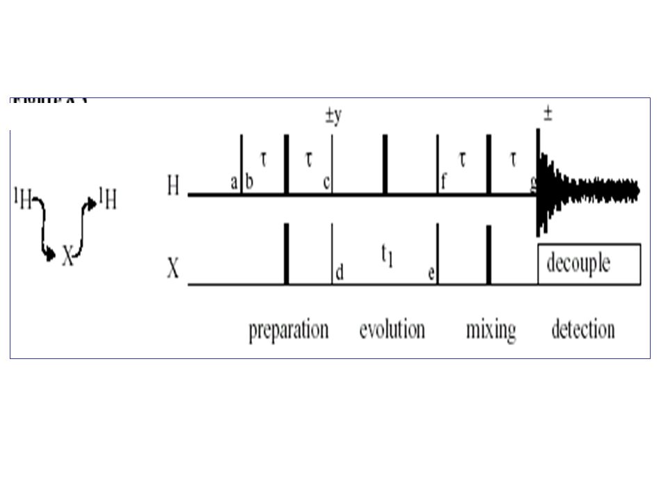
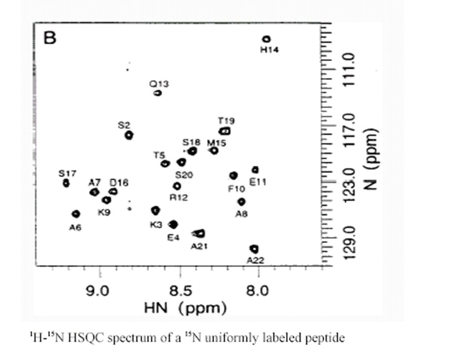
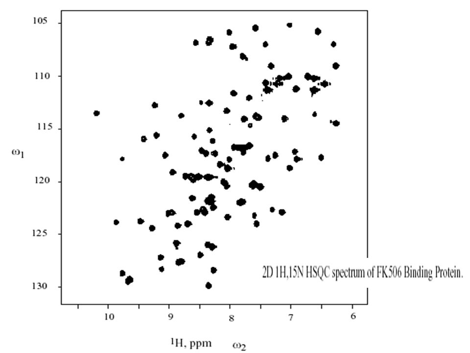
75. HSQC

77. Points a-d (INEPT)

78. Points e-g (Reversed INEPT)

79. Phase Cycling

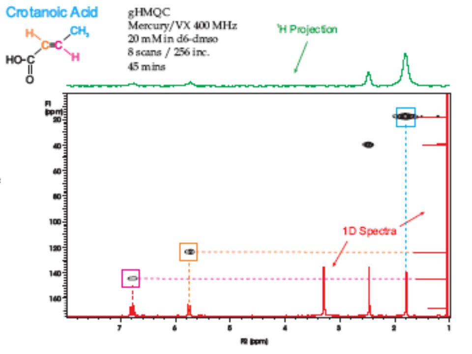
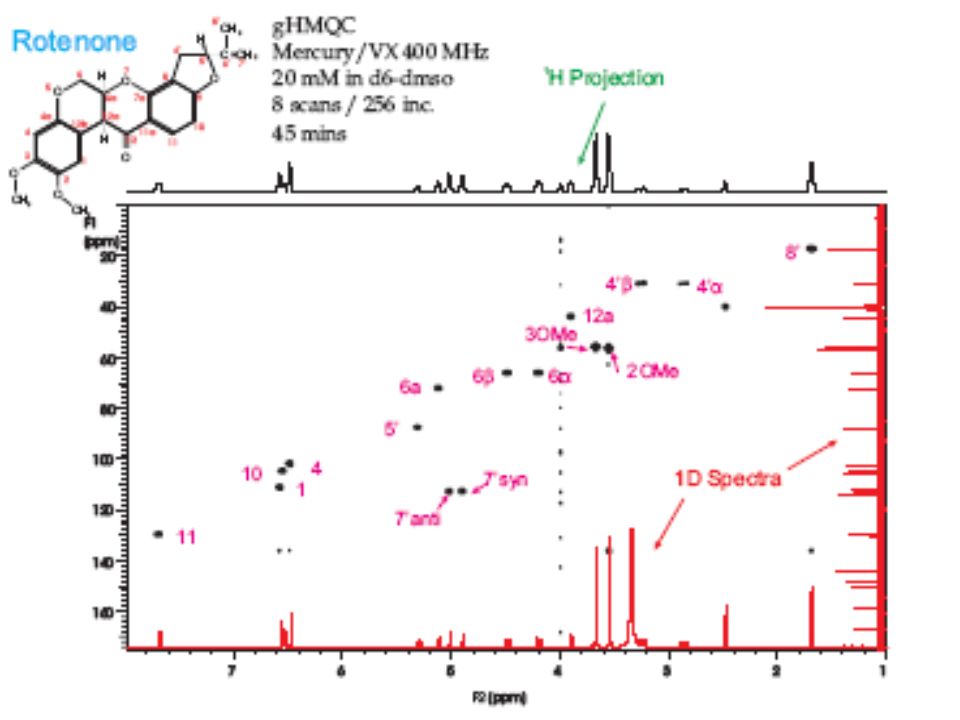
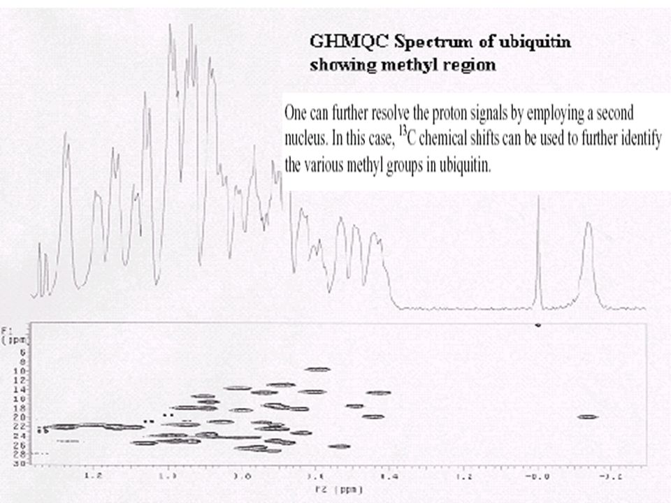
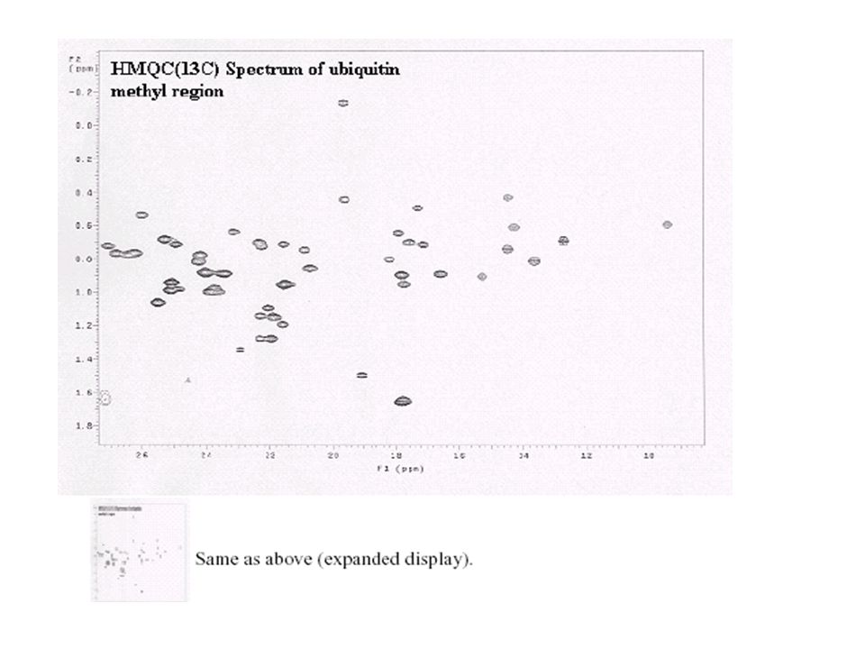
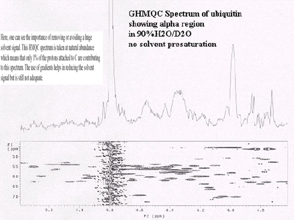
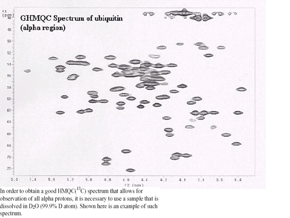
84. HMQC

92. Difference of HMQC and HSQC(I)

93. Difference of HMQC and HSQC(II)

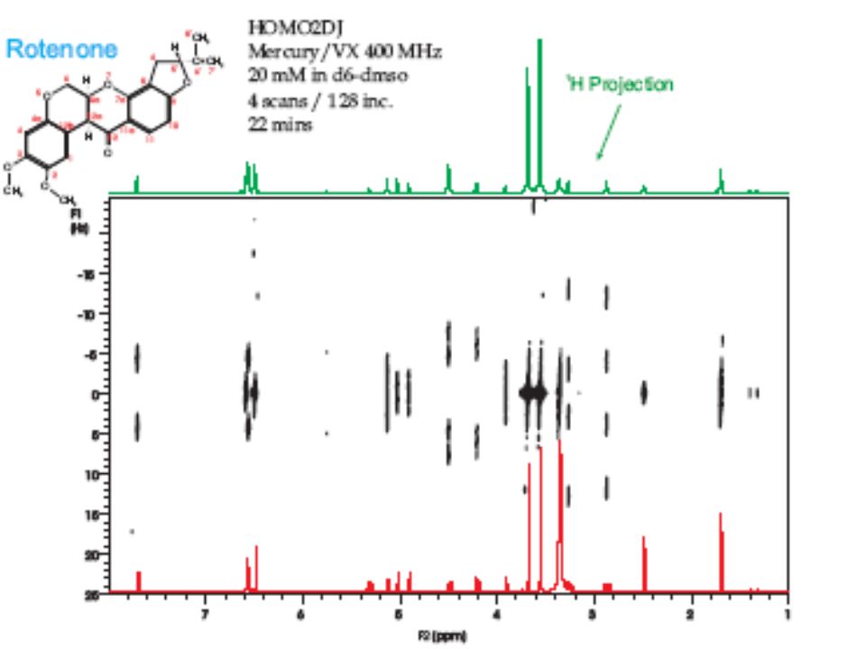
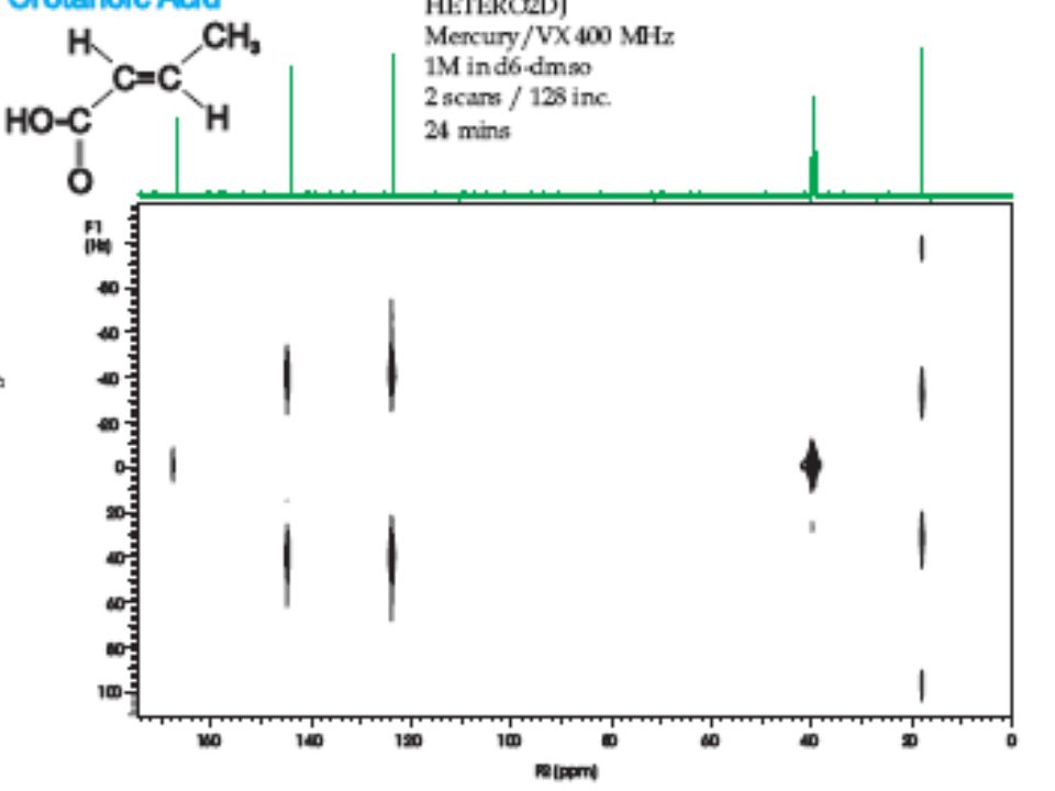
94. 2D J Spectroscopy 2D methods that show coupling multiplets
versus chemical shift. There is both a
homonuclear and a heteronuclear version.
Both methods are useful for resolving
overlapping multiplets. They are also used to
measure coupling constants. These sequences
allow both J coupling and chemical shift
evolution but re-focus the chemical shifts like a
spin echo sequence ( acq).

95. t1: J; t2: J+CS
t1: JIS, t2: JIS+CSS

100. Summary HETCOR, COLOC HMBC HSQC/HMQC J spectrosc.
HSQC is now a “platform” for many more complicated pulse sequences.