1. What is the likelihood that your model is wrong? Generalized tests and corrections for overdispersion during model fitting and exploration James Thorson, Kelli Johnson, Richard Methot, and Ian Taylor Oct. 20, 2015 NWFSC (Seattle)

2. Outline Likelihoods and random processes Surplus production model Steps for real-world assessments 1.Standardizing compositional data for input sample size 2.Estimating effective sample size 3.Exploring process errors for overdispersed fleets Plan moving forward – Probability of the model given data

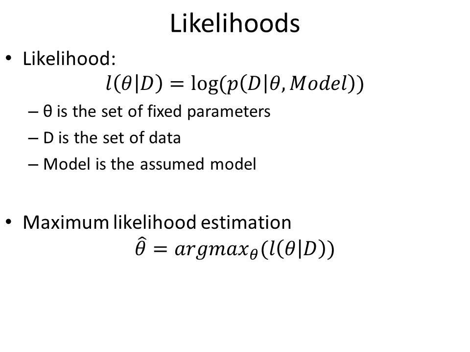
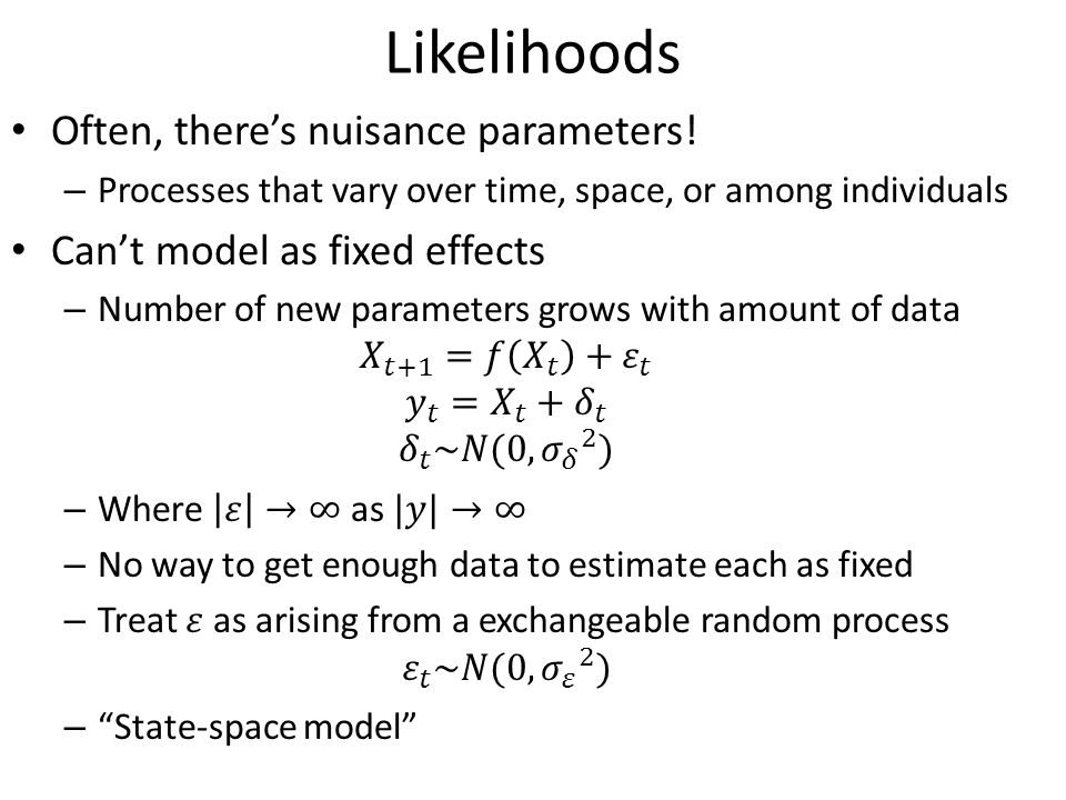
3. Likelihoods

9. Implications 1.If you want to estimate fixed effects …. 2.… and there’s additional stochastic process that is unobservable… 3.… then you can estimate fixed-effects via a mixed- effects model! Benefits – Generic approach to correlations, heteroskedasticity, and heterogeneity – (Fixes most violations in statistical models)

10. Likelihoods Hierarchical models Why would you make a hierarchy of parameters? 1.Stein’s paradox and shrinkage – Pooling parameters towards a mean will be more accurate on average 2.Biological intuition – Formulate models based on knowledge of constituent parts 3.Variance partitioning – Separate different sources of variability (e.g., measurement errors!) More reading – Thorson, J.T., Minto, C., 2015. Mixed effects: a unifying framework for statistical modelling in fisheries biology. ICES J. Mar. Sci. J. Cons. 72, 1245–1256. – https://github.com/james-thorson/mixed-effects https://github.com/james-thorson/mixed-effects

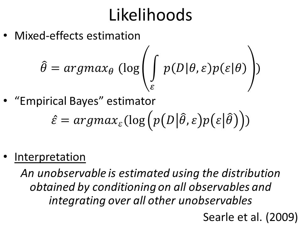
11. Likelihoods

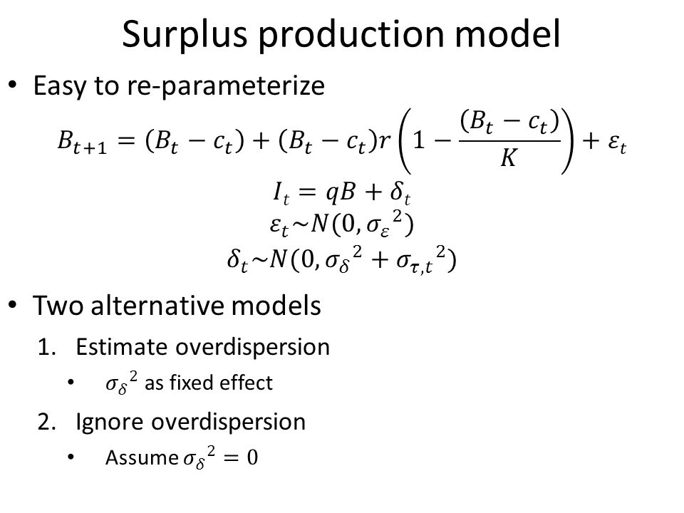
12. Surplus production model

14. Restrictions – Assume r is known – (Otherwise scale K is confounded with productivity r) Programming techniques – Explicit-F parameterization – Treat exploitation rate as random effect, with variance fixed at low value (CV=0.01) Code publicly available: https://github.com/James- Thorson/state_space_production_model

15. Estimating overdispersion Neglecting overdispersion Surplus production model

16. Accounting for overdispersion improves parameter estimates (estimate, ignore, true)

17. Step #1: Comp. standardization Three sampling “Strata”: latitude Difference in age-structure by depth Thorson, J.T., 2014. Standardizing compositional data for stock assessment. ICES J. Mar. Sci. J. Cons. 71, 1117–1128.

18. Step #1: Comp. standardization

19. Difference in age structure by depth Dotted: inshore Dashed: offshore Solid: combined

20. Step #1: Comp. standardization Four estimators Design-based Dirichlet-multinomial Normal approx. Normal w/ process error Performance for estimating proportion at age Top of panel – RMSE, low is good – (bias), close to zero is good

21. Step #1: Comp. standardization Estimating overdispersion Dirichlet-multinomial Normal approx. Normal w/ process error

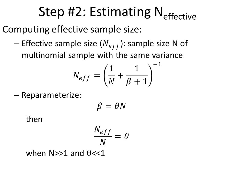
22. Step #2: Estimating N effective Modify Stock Synthesis V3.3 – target release date: Jan. 2016 New feature: Dirichlet-multinomial distribution – Turn-on for any fleet (fishery or survey) – Works for length/age comps – Should work for conditional age-at-length and length-at- age (but is not tested) – Allows mirroring (single parameter for multiple fleets) Useful for spatially stratified models (e.g., Canary rockfish)

23. Step #2: Estimating N effective

25. Linear effective sample size New parameter has similar action to iterative- reweighting factors Therefore… Compare its performance with McAllister-Ianelli iterative reweighting approach

26. Step #2: Estimating N effective Factorial design Three levels of overdispersion Three true sample sizes (N={25,100,400}) Conclusion Dirichlet-multinomial estimates N eff accurately – Small positive bias given high true sample size

27. Step #2: Estimating N effective Performance for estimating parameters? – Works similarly to McAllister-Ianelli method Estimation method True overdispersion

28. Step #2: Estimating N effective Case study: pacific hake – Four models: Unweighted, McAllister-Ianelli, Dirichlet-multinomial, no fishery ages Conclusion: Works similarly to McAllister-Ianelli

29. Step #2: Estimating N effective Benefits of internal estimation 1.Allows proper weighting during profiles and sensitivities – Profiles/sensitivities currently aren’t often tuned 2.Propagates uncertainty during standard errors and forecast intervals – Uncertainty in weighting currently not included in any confidence/credible intervals 3.Permits focus on other iterative model-fitting steps – Variance of process errors!

30. Step #3: Process errors Many methods to estimate process errors in assessment models 1.Add a penalty and “wing it” Just call it “penalized likelihood” and hope no one asks… Eye-ball fit to data Ad hoc tuning 2.First-order approximations Statistically motivated tuning (G. Thompson, pers. comm.) Sample variance plus estimation variance (Methot and Taylor 2014, CJFAS) 3.Clever model modifications Empirical weight-at-age 4.Statistical methods Laplace approximation (Thorson Hicks Methot 2014 ICESJMS) Bayesian estimation (e.g., Mäntyniemi et al. 2013 CJFAS)

31. Step #3: Process errors Laplace approximation 1.ADMB – very slow Requires iterative re-fitting of model 2.TMB – fast and efficient Requires rebuilding code

32. Step #3: Process errors Template Model Builder – Permits faster estimation with more parameters Fully spatial delay-difference model – Accounts for spatial variation in spawning biomass Thorson, J.T., Ianelli, J., Munch, S., Ono, K., Spencer, P., In press. Spatial delay-difference modelling: a new approach to estimating spatial and temporal variation in recruitment and population abundance. Can. J. Fish. Aquat. Sci.

33. Step #3: Process errors Clever model modifications 1.Empirical weight-at-age Deals easily with time-varying growth Doesn’t account for uncertainty 2.Statistical VPA (MacCall and Teo 2013 Fish Res) Deals with time-varying selectivity Not easy in most software packages 3.Empirical maturity and fecundity schedules (I think this is still the norm most places…)

34. Plan moving forward Three practical steps: 1.Estimate input sample sizes from the data 2.Account for overdispersion as a parameter 3.Account for correlations via process errors Why not combine steps 2 and 3?

35. Plan moving forward Why not combine Steps 2 and 3? – Structure of correlation in fishery models is very complicated! Correlations among: 1.ages 2.lengths 3.sexes 4.fleets – There’s probably many ways to model correlations Different methods account for some correlations but not others! Francis (2014) account for correlations among lengths OR ages, but not simultaneously

36. Plan moving forward Obvious approach to modelling correlations… … is mixed effects! Benefits 1.Retains focus on modelling the process Doesn’t obfuscate correlations 2.Allows calculation of predicted compositions Hard to calculate using methods that use ad hoc corrections for correlations 3.Keeps us working with mainstream statistics Easier to work with ecologists E.g., U-CARE and E-SURGE as diagnostic for overdispersion in tag-resighting models

37. Plan moving forward Where can we start? Make a list of unmodeled processes that generate correlations in compositional data – Recruitment variation (usually modeled explicitly) – Time-varying selectivity (Actually caused by spatial variation in density and fishing rate) – Time-varying individual growth – Time- and age-varying natural mortality rates

38. Plan moving forward What if there’s multiple processes that can account for correlations? Multi-model inference 1.Model selection Only valid if each constituent model is admissible 2.Model averaging / Ensemble modelling Averaging results from multiple models 3.Multi-model decision theory Averaging decision from each model, with weights derived for performance in that decision

39. Plan moving forward Next steps 1.Methods and software for compositional standardization Big black-box in most assessments I’ve seen! 2.Additional research regarding internal estimation of overdispersion Does it affect estimates of uncertainty? Does it affect profiles? 3.Improved algorithms and software for mixed-effect assessment models

40. Acknowledgements Input on themes – Allan Hicks, Mark Maunder