2. Lecturer’s desk Physics- atmospheric Sciences (PAS) - Room 201 s c r e e n Row A Row B Row C Row D Row E Row F Row G Row H 131211109 87 Row A 14131211109 87 Row B 1514131211109 87 Row C 1514131211109 87 Row D 16 1514131211109 87 Row E 17 16 1514131211109 87 Row F 1716 1514131211109 87 Row G 1716 1514131211109 87 Row H 16 18 table Row A Row B Row C Row D Row E Row F Row G Row H 15141716 1819 16 15 18171920 17161918 2021 18172019 2122 19182120 2223 20192221 2324 18172019 2122 19182120 2223 2143 56 2143 56 2143 56 2143 56 2143 56 2143 56 2143 56 2143 56 Row J Row K Row L Row M Row N Row P 2143 5 2143 5 2143 5 2143 5 2143 5 1 5 Row J Row K Row L Row M Row N Row P 27262928 30 25242726 28 24232625 27 23222524 26 25242726 28 27262928 30 6 14 131211109 87 16151817 19 202122 614131211109 87 16 15 18 17 19 20212223 614131211109 87 16 15 18171920 2122 23 6 14 131211109 87 1624181719 20 2122 231525 6 14 131211109 87 1624181719 20 2122 231525 Row Q 2143 5 27262928 30 6 14 131211109 87 242223 21 - 15 25 37363938 40 34 3132 3335 69 87 13 table 14 18 192021

3. MGMT 276: Statistical Inference in Management Fall 2015

5. Before our next exam (November 10 th ) OpenStax Chapters 1 – 10 and Chapter 13 Plous (2, 3, & 4) Chapter 2: Cognitive Dissonance Chapter 3: Memory and Hindsight Bias Chapter 4: Context Dependence Schedule of readings

6. On class website: Please print and complete homework worksheet #14 Hypothesis testing using ANOVAs Due: Thursday November 5 th Homework

7. Logic of hypothesis testing Steps for hypothesis testing Levels of significance (Levels of alpha) what does p < 0.05 mean? what does p < 0.01 mean? Hypothesis testing with t-scores (two independent samples) Analysis of Variance (ANOVA) Constructing brief, complete summary statements By the end of lecture today 11/3/15

8. Exam 3 – Tuesday (11/10/14) Bring 2 calculators (remember only simple calculators, we can’t use calculators with programming functions) Bring 2 pencils (with good erasers) Bring ID Stats Review by Nick and Jonathon When: Monday evening November 9 th - 6:30 – 7:50pm Where: ILC 130 Cost: $5.00 Stats Review by Nick and Jonathon When: Monday evening November 9 th - 6:30 – 7:50pm Where: ILC 130 Cost: $5.00

9. Just for Fun Assignments Go to D2L - Click on “Content” Click on “Interactive Online Just-for-fun Assignments” Please note: These are not worth any class points and are different from the required homeworks

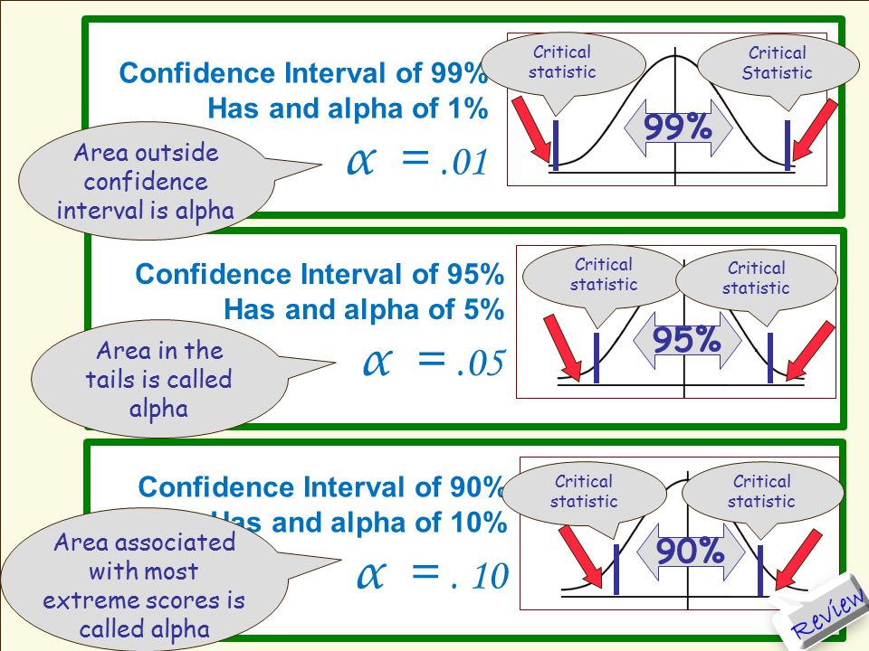
11. Confidence Interval of 99% Has and alpha of 1% α =.01 Confidence Interval of 90% Has and alpha of 10% α =. 10 Confidence Interval of 95% Has and alpha of 5% α =.05 99%95%90% Area outside confidence interval is alpha Area in the tails is called alpha Area associated with most extreme scores is called alpha Critical statistic Critical Statistic Critical statistic Critical statistic Critical statistic Critical statistic

12. Rejecting the null hypothesis The result is “statistically significant” if: the observed statistic is larger than the critical statistic (which can be a ‘z” or “t” or “r” or “F” or x 2 ) observed stat > critical stat If we want to reject the null, we want our t (or z or r or F or x 2 ) to be big!! the p value is less than 0.05 (which is our alpha) p < 0.05 If we want to reject the null, we want our “p” to be small!! we reject the null hypothesis then we have support for our alternative hypothesis

13. Independent samples t-test Donald is a consultant and leads training sessions. As part of his training sessions, he provides the students with breakfast. He has noticed that when he provides a full breakfast people seem to learn better than when he provides just a small meal (donuts and muffins). So, he put his hunch to the test. He had two classes, both with three people enrolled. The one group was given a big meal and the other group was given only a small meal. He then compared their test performance at the end of the day. Please test with an alpha =.05 Big Meal 22 25 Small meal 19 23 21 Mean= 24 Mean= 21 Are the two means significantly different from each other, or is the difference just due to chance? Rev iew

14. The mean test score for participants who ate the big meal was 24, while the mean test score for participants who ate the small meal was 21. A t-test was completed and there appears to be no significant difference in the test scores as a function of the size of the meal, t(4) = 1.96; n.s. Start summary with two means (based on DV) for two levels of the IV Describe type of test (t-test versus anova) with brief overview of results Finish with statistical summary t(4) = 1.96; ns Type of test with degrees of freedom Value of observed statistic n.s. = “not significant” p<0.05 = “significant”

15. Independent samples t-test Donald is a consultant and leads training sessions. As part of his training sessions, he provides the students with breakfast. He has noticed that when he provides a full breakfast people seem to learn better than when he provides just a small meal (donuts and muffins). So, he put his hunch to the test. He had two classes, both with three people enrolled. The one group was given a big meal and the other group was given only a small meal. He then compared their test performance at the end of the day. Please test with an alpha =.05 What if we ran more subjects? Big Meal 22 25 22 25 22 25 Small meal 19 23 21 19 23 21 19 23 21 Mean= 24 Mean= 21

16. What happened? We ran more subjects: Increased n So, we decreased variability Easier to find effect significant even though effect size didn’t change Big sampleSmall sample This is variance for each sample (Remember, variance is just standard deviation squared) This is variance for each sample (Remember, variance is just standard deviation squared)

17. If this is less than.05 (or whatever alpha is) it is significant, and we the reject null df = (n 1 – 1) + (n 2 – 1) = (165 - 1) + (120 -1) = 283

18. A survey was conducted to see whether men or women superintendents make more money 1.The independent variable is ________________ 2.The dependent variable is _________________ 3. Who made more money men or women? 4. Identify the two means and the observed t score 5. Identify the p value and state whether it is less than.05

19. A survey was conducted to see whether men or women superintendents make more money 1.37834 E-05 Equals.00001378 4 zeros 6.8917 E-06 Equals.0000068917 5 zeros Are both p values less than 0.05?

20. A survey was conducted to see whether men or women superintendents make more money 1.37834 E-05 Equals.00001378 4 zeros 6.8917 E-06 Equals.0000068917 5 zeros A note on scientific notation: “E-05” means move the decimal to the left 5 places E-06” means move the decimal to the left 6 places

21. A survey was conducted to see whether men or women superintendents make more money. The independent variable is a. nominal level of measurement b. ordinal level of measurement c. interval level of measurement d. ratio level of measurement correct

22. A survey was conducted to see whether men or women superintendents make more money. The dependent variable is a. nominal level of measurement b. ordinal level of measurement c. interval level of measurement d. ratio level of measurement correct

23. A survey was conducted to see whether men or women superintendents make more money. The independent variable is a. continuous and qualitative b. continuous and quantitative c. discrete and qualitative d. discrete and quantitative correct

24. A survey was conducted to see whether men or women superintendents make more money. The dependent variable is a. continuous and qualitative b. continuous and quantitative c. discrete and qualitative d. discrete and quantitative correct

25. A survey was conducted to see whether men or women superintendents make more money. This is a a. quasi, between subject design b. quasi, within subject design c. true, between subject design d. true, within subject design correct

26. A survey was conducted to see whether men or women superintendents make more money. This is a a. one-tailed test b. two-tailed test c. three-tailed test d. not enough information correct

27. A survey was conducted to see whether men or women superintendents make more money. The null hypothesis is a. men make more money b. women make more money c. no difference between amount of money made d. there is a difference between the amount of money made correct

28. A survey was conducted to see whether men or women superintendents make more money. If the null hypothesis was rejected we will conclude that a. men make more money b. women make more money c.no difference between amount of money made d. there is a difference between the amount of money made correct

29. A survey was conducted to see whether men or women superintendents make more money. A Type I error would be a. claiming men make more money, when they don’t b. claiming women make more money, when they don’t c.claiming no difference between amount of money made, when there is a difference d. claiming there is a difference between the amount of money made, when there is no difference correct

30. A survey was conducted to see whether men or women superintendents make more money. A Type II error would be a. claiming men make more money, when they don’t b. claiming women make more money, when they don’t c.claiming no difference between amount of money made, when there is a difference d. claiming there is a difference between the amount of money made, when there is no difference correct

31. An t-test was conducted, there were ___ men in the study and ___ women. a. 18; 21 b. 21; 18 c. 19; 19 d. 38; 38 Let’s try one correct

32. A t-test was conducted, which of the following best describes the results: a. t(37) = 2.02; p < 0.05 b. t(21) = 2.02; n.s. c. t(37) = 5.0; p < 0.05 d. t(21) = 5.0; n.s Let’s try one correct

33. A t-test was conducted, with a two tail test was there a significant difference? a. No, because 5.0 is not bigger than 6.89 b. Yes, because 5.0 is bigger than 1.68. c. Yes, because 5.0 is bigger than 1.37 d. Yes, because 5.0 is bigger than 2.02 Let’s try one correct

34. Which is true a. p < 0.05 b. p < 0.01 c. p < 0.001 d. All of the above Let’s try one correct

35. A survey was conducted to see whether women superintendents make more money than men. This is a a. one-tailed test b. two-tailed test c. three-tailed test d. not enough information Note the change in the problem correct

36. A survey was conducted to see whether women superintendents make more money than men. A t-test was conducted, which of the following best describes the results: Note the results were in the unpredicted direction a. reject the null b. do not reject the null c. not enough information Let’s try one correct

37. A survey was conducted to see whether women superintendents make more money than men. A t-test was conducted, which of the following best describes the results: Note the results were in the unpredicted direction a. t(21) = 2.02; p < 0.05 b. t(21) = 2.02; n.s. c. t(37) = 5.0; p < 0.05 d. t(37) = 5.0; n.s Let’s try one correct

38. Homework review

39. . Homework Is there a difference in mpg between these two cars 2-tail 18 0.05 There is no difference in mpg between these two cars There is a difference in mpg between these two cars

40. α =.05 (df) = 18 Critical t (18) = 2.101 two tail test

41. . Homework Is there a difference in mpg between these two cars 2-tail 18 0.05 2.101 There is no difference in mpg between these two cars There is a difference in mpg between these two cars S 2 pooled = (n 1 – 1) s 1 2 + (n 2 – 1) s 2 2 n 1 + n 2 - 2 =.82 S 2 pooled = (10 – 1) (.80) 2 + (10 – 1) (1) 2 10 1 + 10 2 - 2 = 3.704 t = 17 – 18.5.82/10 +.82/10 = 1.5.4049691

42. . Homework The average mpg is 18.5 for the Ford Explorer and 17.0 for the Expedition. A t-test was conducted and found this difference to be significantly different, t(18) = 3.70; p < 0.05 Yes Is there an increase in foot size from 1960 to 1980 Is there no difference (or a decrease) in foot size from 1960 to 1980 There is an increase in foot size from 1960 to 1980 2-tail 22 0.05

43. α =.05 (df) = 22 Critical t (22) = 1.717 one tail test

44. . Homework The average mpg is 18.5 for the Ford Explorer and 17.0 for the Expedition. A t-test was conducted and found this difference to be significantly different, t(18) = 3.70; p < 0.05 Yes Is there an increase in foot size from 1960 to 1980 Is there no difference (or a decrease) in foot size from 1960 to 1980 There is an increase in foot size from 1960 to 1980 2-tail 22 0.05 1.717

45. . Homework Yes =.6201 =.4502 =.2936 S 2 pooled = (12 – 1) (.6201) 2 + (12 – 1) (4502) 2 12 1 + 12 2 - 2 = 2.26 t = 8.208 – 7.708.2936/12 +.2936/12 = 0.5.2212 Yes The average foot size for women in 1960 is 7.7, while the average foot size for women in 1980 is 8.2. A t-test was conducted and found that the increase in foot size is statistically significant, t(22) = 2.26; p < 0.05

46. . Homework

47. .

48. . Type of instruction Exam score 50 0.05 2-tail 2.66 2.02 40 38 p = 0.0113 yes CAUTION This is significant with alpha of 0.05 BUT NOT WITH alpha of 0.01 The average exam score for those with instruction was 50, while the average exam score for those with no instruction was 40. A t-test was conducted and found that instruction significantly improved exam scores, t(38) = 2.66; p < 0.05

49. . Homework Type of Staff Travel Expenses 142.5 0.05 2-tail 1.53679 2.2 130.29 11 p = 0.153 no The average expenses for sales staff is 142.5, while the average expenses for the audit staff was 130.29. A t-test was conducted and no significant difference was found, t(11) = 1.54; n.s.

50. . Homework Location of lot Number of cars 86.24 0.05 2-tail -0.88 2.01 92.04 51 p = 0.38 no The average number of cars in the Ocean Drive Lot was 86.24, while the average number of cars in Rio Rancho Lot was 92.04. A t-test was conducted and no significant difference between the number of cars parked in these two lots, t(51) = -.88; n.s. Fun fact: If the observed t is less than one it will never be significant

51. Study Type 2: t-test Study Type 3: One-way Analysis of Variance (ANOVA) Comparing more than two means We are looking to compare two means

52. Single Independent Variable comparing more than two groups Study Type 3: One-way ANOVA Single Dependent Variable (numerical/continuous) Independent Variable: Type of incentive Levels of Independent Variable: None, Bike, Trip to Hawaii Dependent Variable: Number of cookies sold Levels of Dependent Variable: 1, 2, 3 up to max sold Between participant design Causal relationship: Incentive had an effect – it increased sales Ian was interested in the effect of incentives for girl scouts on the number of cookies sold. He randomly assigned girl scouts into one of three groups. The three groups were given one of three incentives and looked to see who sold more cookies. The 3 incentives were 1) Trip to Hawaii, 2) New Bike or 3) Nothing. This is an example of a true experiment Used to test the effect of the IV on the DV How could we make this a quasi-experiment?

53. Single Independent Variable comparing more than two groups Study Type 3: One-way ANOVA Single Dependent Variable (numerical/continuous) Ian was interested in the effect of incentives for girl scouts on the number of cookies sold. He randomly assigned girl scouts into one of three groups. The three groups were given one of three incentives and looked to see who sold more cookies. The 3 incentives were 1) Trip to Hawaii, 2) New Bike or 3) Nothing. This is an example of a true experiment Used to test the effect of the IV on the DV None New Bike Sales per Girl scout Trip Hawaii None New Bike Trip Hawaii Dependent variable is always quantitative In an ANOVA, independent variable is qualitative (& more than two groups) Sales per Girl scout

54. One-way ANOVA One-way ANOVAs test only one independent variable - although there may be many levels “Factor” = one independent variable “Level” = levels of the independent variable treatment condition groups “Main Effect” of independent variable = difference between levels Note: doesn’t tell you which specific levels (means) differ from each other A multi-factor experiment would be a multi-independent variables experiment Number of cookies sold Incentives None Bike Hawaii trip

55. Comparing ANOVAs with t-tests Similarities still include: Using distributions to make decisions about common and rare events Using distributions to make inferences about whether to reject the null hypothesis or not The same 5 steps for testing an hypothesis The three primary differences between t-tests and ANOVAS are: 1. ANOVAs can test more than two means 2. We are comparing sample means indirectly by comparing sample variances 3. We now will have two types of degrees of freedom t(16) = 3.0; p < 0.05 F(2, 15) = 3.0; p < 0.05 Tells us generally about number of participants / observations Tells us generally about number of groups / levels of IV

56. A girl scout troop leader wondered whether providing an incentive to whomever sold the most girl scout cookies would have an effect on the number cookies sold. She provided a big incentive to one troop (trip to Hawaii), a lesser incentive to a second troop (bicycle), and no incentive to a third group, and then looked to see who sold more cookies. n = 5 x = 10 n = 5 x = 12 n = 5 x = 14 Troop 1 (nada) 10 8 12 7 13 Troop 2 (bicycle) 12 14 10 11 13 Troop 3 (Hawaii) 14 9 19 13 15 What is Independent Variable? How many groups? What is Dependent Variable? How many levels of the Independent Variable?

57. Main effect of incentive: Will offering an incentive result in more girl scout cookies being sold? If we have a “effect” of incentive then the means are significantly different from each other we reject the null we have a significant F p < 0.05 We don’t know which means are different from which …. just that they are not all the same To get an effect we want: Large “F” - big effect and small variability Small “p” - less than 0.05 (whatever our alpha is)

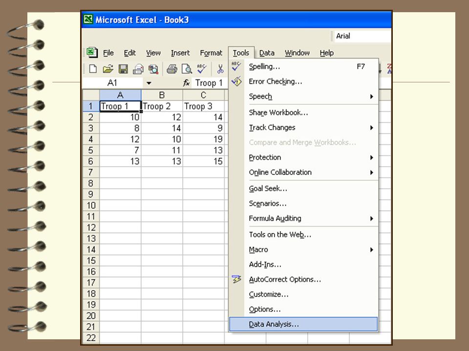
58. Let ’ s do same problem Using MS Excel A girlscout troop leader wondered whether providing an incentive to whomever sold the most girlscout cookies would have an effect on the number cookies sold. She provided a big incentive to one troop (trip to Hawaii), a lesser incentive to a second troop (bicycle), and no incentive to a third group, and then looked to see who sold more cookies. Troop 1 (Nada) 10 8 12 7 13 Troop 2 (bicycle) 12 14 10 11 13 Troop 3 (Hawaii) 14 9 19 13 15 n = 5 x = 10 n = 5 x = 12 n = 5 x = 14

59. Let ’ s do same problem Using MS Excel

61. Let ’ s do one Replication of study (new data)

62. Let ’ s do same problem Using MS Excel

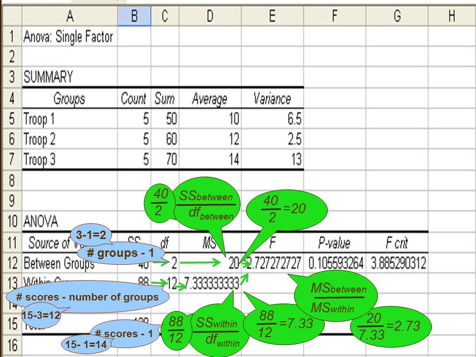
64. SS within df within SS between df between 88 12 =7.33 40 2 =20 20 7.33 =2.73 40 2 88 12 MS between MS within # groups - 1 # scores - number of groups # scores - 1 3-1=2 15-3=12 15- 1=14

65. F critical (is observed F greater than critical F?) P-value (is it less than.05?) No, so it is not significant Do not reject null No, so it is not significant Do not reject null

66. Make decision whether or not to reject null hypothesis 2.7 is not farther out on the curve than 3.89 so, we do not reject the null hypothesis Observed F = 2.73 Critical F (2,12) = 3.89 Also p-value is not smaller than 0.05 so we do not reject the null hypothesis Step 6: Conclusion: There appears to be no effect of type of incentive on number of girl scout cookies sold

67. Make decision whether or not to reject null hypothesis 2.7 is not farther out on the curve than 3.89 so, we do not reject the null hypothesis Observed F = 2.72727272 Critical F (2,12) = 3.88529 Conclusion: There appears to be no effect of type of incentive on number of girl scout cookies sold F (2,12) = 2.73; n.s. The average number of cookies sold for three different incentives were compared. The mean number of cookie boxes sold for the “Hawaii” incentive was 14, the mean number of cookies boxes sold for the “Bicycle” incentive was 12, and the mean number of cookies sold for the “No” incentive was 10. An ANOVA was conducted and there appears to be no significant difference in the number of cookies sold as a result of the different levels of incentive F(2, 12) = 2.73; n.s.