1. Class 12: Barabasi-Albert Model-Part II Prof. Albert-László Barabási Dr. Baruch Barzel, Dr. Mauro Martino Network Science: Evolving Network Models February 2015 Prof. Boleslaw Szymanski

2. A.-L.Barabási, R. Albert and H. Jeong, Physica A 272, 173 (1999) Number of nodes with degree k at time t. Nr. of degree k-1 nodes that acquire a new link, becoming degree k Preferential attachment Since at each timestep we add one node, we have N=t (total number of nodes = number of timesteps) 2m: each node adds m links, but each link contributed to the degree of 2 nodes Number of links added to degree k nodes after the arrival of a new node: Total number of k-nodes New node adds m new links to other nodes Nr. of degree k nodes that acquire a new link, becoming degree k+1 # k-nodes at time t+1 # k-nodes at time t Gain of k- nodes via k-1  k Loss of k- nodes via k  k+1 MFT - Degree Distribution: Rate Equation

3. A.-L.Barabási, R. Albert and H. Jeong, Physica A 272, 173 (1999) # m-nodes at time t+1 # m- nodes at time t Add one m-degeree node Loss of an m-node via m  m+1 We do not have k=0,1,...,m-1 nodes in the network (each node arrives with degree m)  We need a separate equation for degree m modes # k-nodes at time t+1 # k-nodes at time t Gain of k- nodes via k-1  k Loss of k- nodes via k  k+1 MFT - Degree Distribution: Rate Equation Network Science: Evolving Network Models February 2015

4. k>m We assume that there is a stationary state in the N=t  ∞ limit, when P(k,∞)=P(k) k>m MFT - Degree Distribution: Rate Equation Network Science: Evolving Network Models February 2015

5. ... m+3  k Krapivsky, Redner, Leyvraz, PRL 2000 Dorogovtsev, Mendes, Samukhin, PRL 2000 Bollobas et al, Random Struc. Alg. 2001 for large k MFT - Degree Distribution: Rate Equation Network Science: Evolving Network Models February 2015

6. Its solution is: Start from eq. Dorogovtsev and Mendes, 2003 MFT - Degree Distribution: A Pretty Caveat Network Science: Evolving Network Models February 2015

7. γ = 3 Network Science: Evolving Network Models Degree distribution (i) The degree exponent is independent of m. (ii) As the power-law describes systems of rather different ages and sizes, it is expected that a correct model should provide a time-independent degree distribution. Indeed, asymptotically the degree distribution of the BA model is independent of time (and of the system size N)  the network reaches a stationary scale-free state. (iii) The coefficient of the power-law distribution is proportional to m 2. for large k

8. NUMERICAL SIMULATION OF THE BA MODEL

9. Absence of growth or preferential attachment Section 6

10. growth preferential attachment Π(k i ) : uniform MODEL A Network Science: Evolving Network Models February 2015

11. growth preferential attachment P(k) : power law (initially)  Gaussian  Fully Connected MODEL B Network Science: Evolving Network Models February 2015

12. Do we need both growth and preferential attachment? YEP. Network Science: Evolving Network Models February 2015

13. P(k) ~ k -  Regular network Erdos- Renyi Watts- Strogatz P(k)=δ(k-k d ) Exponential Barabasi- Albert P(k) ~ k -  EMPIRICAL DATA FOR REAL NETWORKS Pathlenght Clustering Degree Distr. Network Science: Evolving Network Models February 2015

14. Diameter and clustering coefficient Section 10

15. Distances in scale-free networks Size of the biggest hub is of order O(N). Most nodes can be connected within two layers of it, thus the average path length will be independent of the system size. The average path length increases slower than logarithmically. In a random network all nodes have comparable degree, thus most paths will have comparable length. In a scale-free network the vast majority of the path go through the few high degree hubs, reducing the distances between nodes. Some key models produce γ=3, so the result is of particular importance for them. This was first derived by Bollobas and collaborators for the network diameter in the context of a dynamical model, but it holds for the average path length as well. The second moment of the distribution is finite, thus in many ways the network behaves as a random network. Hence the average path length follows the result that we derived for the random network model earlier. Cohen, Havlin Phys. Rev. Lett. 90, 58701(2003); Cohen, Havlin and ben-Avraham, in Handbook of Graphs and Networks, Eds. Bornholdt and Shuster (Willy-VCH, NY, 2002) Chap. 4; Confirmed also by: Dorogovtsev et al (2002), Chung and Lu (2002); (Bollobas, Riordan, 2002; Bollobas, 1985; Newman, 2001 Small World DISTANCES IN SCALE-FREE NETWORKS

16. Section 10 Diameter Bollobas, Riordan, 2002

17. P(k) ~ k -  P(k)=δ(k-k d ) Exponential P(k) ~ k -  EMPIRICAL DATA FOR REAL NETWORKS Pathlenght Clustering Degree Distr. Regular network Erdos- Renyi Watts- Strogatz Barabasi- Albert Network Science: Evolving Network Models February 2015

18. Section 10 Clustering coefficient What is the functional form of C(N)? Reminder: for a random graph we have: Konstantin Klemm, Victor M. Eguiluz, Growing scale-free networks with small-world behavior, Phys. Rev. E 65, 057102 (2002), cond-mat/0107607

19. 1 2 Denote the probability to have a link between node i and j with P(i,j) The probability that three nodes i,j,l form a triangle is P(i,j)P(i,l)P(j,l) The expected number of triangles in which a node l with degree k l participates is thus: We need to calculate P(i,j). CLUSTERING COEFFICIENT OF THE BA MODEL Network Science: Evolving Network Models February 2015

20. Calculate P(i,j). Node j arrives at time t j =j and the probability that it will link to node i with degree k i already in the network is determined by preferential attachment: Where we used that the arrival time of node j is t j =j and the arrival time of node is t i =i Let us approximate: Which is the degree of node l at current time, at time t=N There is a factor of two difference... Where does it come from? CLUSTERING COEFFICIENT OF THE BA MODEL Network Science: Evolving Network Models February 2015

21. CLUSTERING COEFFICIENT OF THE BA MODEL Konstantin Klemm, Victor M. Eguiluz, Phys. Rev. E 65, 057102 (2002) Network Science: Evolving Network Models February 2015

22. P(k) ~ k -  EMPIRICAL DATA FOR REAL NETWORKS Pathlenght Clustering Degree Distr. P(k)=δ(k-k d ) Exponential P(k) ~ k -  Regular network Erdos- Renyi Watts- Strogatz Barabasi- Albert Network Science: Evolving Network Models February 2015

23. Nonlinear preferential attachment Section 8

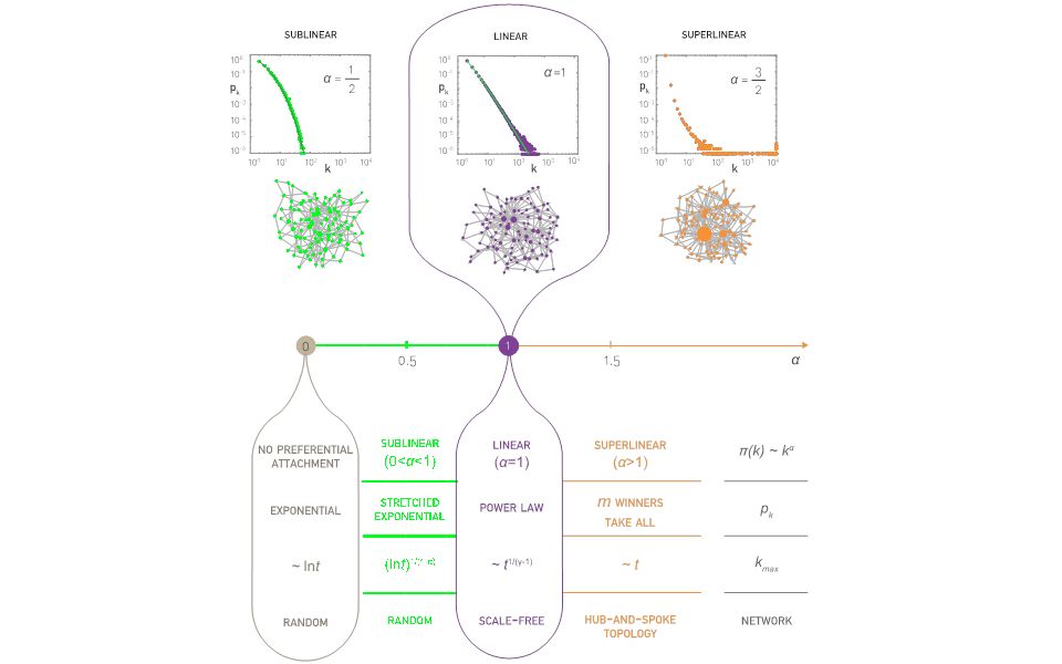
24. Section 8 Nonlinear preferential attachment α=0: Reduces to Model A discussed in Section 5.4. The degree distribution follows the simple exponential function. α=1: Barabási-Albert model, a scale-free network with degree exponent 3. 0<α<1: Sublinear preferential attachment. New nodes favor the more connected nodes over the less connected nodes. Yet, for the bias is not sufficient to generate a scale-free degree distribution. Instead, in this regime the degrees follow the stretched exponential distribution:

25. Section 8 Nonlinear preferential attachment α=0: Reduces to Model A discussed in Section 5.4. The degree distribution follows the simple exponential function. α=1: Barabási-Albert model, a scale-free network with degree exponent 3. α>1: Superlinear preferential attachment. The tendency to link to highly connected nodes is enhanced, accelerating the “rich-gets-richer” process. The consequence of this is most obvious for, when the model predicts a winner-takes-all phenomenon: almost all nodes connect to a single or a few super-hubs.

26. Section 8 Nonlinear preferential attachment The growth of the hubs. The nature of preferential attachment affects the degree of the largest node. While in a scale-free network the biggest hub grows as (green curve), for sublinear preferential attachment this dependence becomes logarithmic (red curve). For superlinear preferential attachment the biggest hub grows linearly with time, always grabbing a finite fraction of all links (blue curve)). The symbols are provided by a numerical simulation; the dotted lines represent the analytical predictions.

28. The origins of preferential attachment Section 9

29. Section 9 Link selection model Link selection model -- perhaps the simplest example of a local or random mechanism capable of generating preferential attachment. Growth: at each time step we add a new node to the network. Link selection: we select a link at random and connect the new node to one of nodes at the two ends of the selected link. To show that this simple mechanism generates linear preferential attachment, we write the probability that the node at the end of a randomly chosen link has degree k as

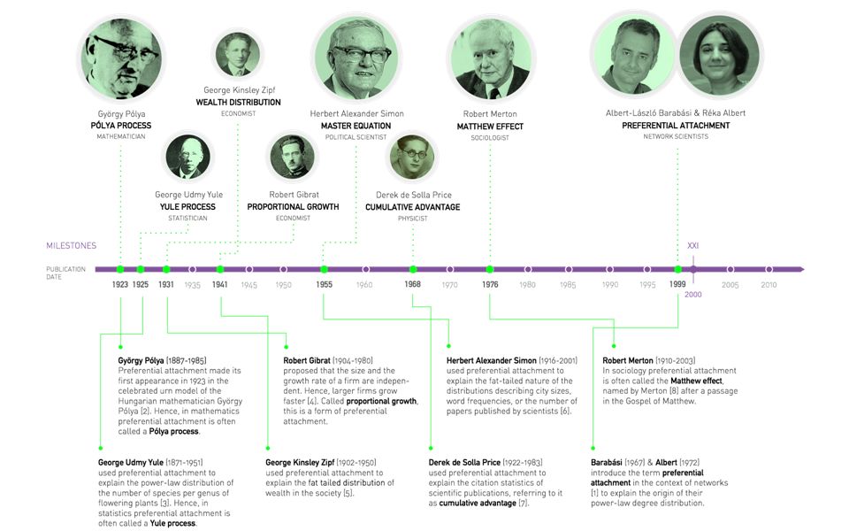
30. Section 9 Originators of preferential attachments

32. Measuring preferential attachment Section 7

33. Section 7 Measuring preferential attachment Plot the change in the degree Δk during a fixed time Δt for nodes with degree k. (Jeong, Neda, A.-L. B, Europhys Letter 2003; cond-mat/0104131) No pref. attach: κ~k Linear pref. attach: κ~k 2 To reduce noise, plot the integral of Π(k) over k: Network Science: Evolving Network Models

34. neurosci collab actor collab. citation network Plots shows the integral of Π(k) over k: Internet Network Science: Evolving Network Models Section 7Measuring preferential attachment No pref. attach: κ~k Linear pref. attach: κ~k 2

35. 1.Copying mechanism directed network select a node and an edge of this node attach to the endpoint of this edge 2.Walking on a network directed network the new node connects to a node, then to every first, second, … neighbor of this node 3.Attaching to edges select an edge attach to both endpoints of this edge 4.Node duplication duplicate a node with all its edges randomly prune edges of new node MECHANISMS RESPONSIBLE FOR PREFERENTIAL ATTACHMENT Network Science: Evolving Network Models February 2015

36. Section 9 Copying model (a) Random Connection: with probability p the new node links to u. (b) Copying: with probability we randomly choose an outgoing link of node u and connect the new node to the selected link's target. Hence the new node “copies” one of the links of an earlier node (a) the probability of selecting a node is 1/N. (b) is equivalent with selecting a node linked to a randomly selected link. The probability of selecting a degree-k node through the copying process of step (b) is k/2L for undirected networks. The likelihood that the new node will connect to a degree-k node follows preferential attachment Social networks: Copy your friend’s friends. Citation Networks: Copy references from papers we read. Protein interaction networks: gene duplication,

37. Proteins with more interactions are more likely to obtain new links: Π(k)~k (preferential attachment) Wagner 2001; Vazquez et al. 2003; Sole et al. 2001; Rzhetsky & Gomez 2001; Qian et al. 2001; Bhan et al. 2002. ORIGIN OF THE SCALE-FREE TOPOLOGY IN THE CELL: Gene Duplication Network Science: Evolving Network Models February 2015

38.  k vs. k : increase in the No. of links in a unit time No PA:  k is independent of k PA:  k ~k Eisenberg E, Levanon EY, Phys. Rev. Lett. 2003 Jeong, Neda, A.-L.B, Europhys. Lett. 2003 PREFERENTIAL ATTACHMENT IN PROTEIN INTERACTION NETWORKS Network Science: Evolving Network Models February 2015

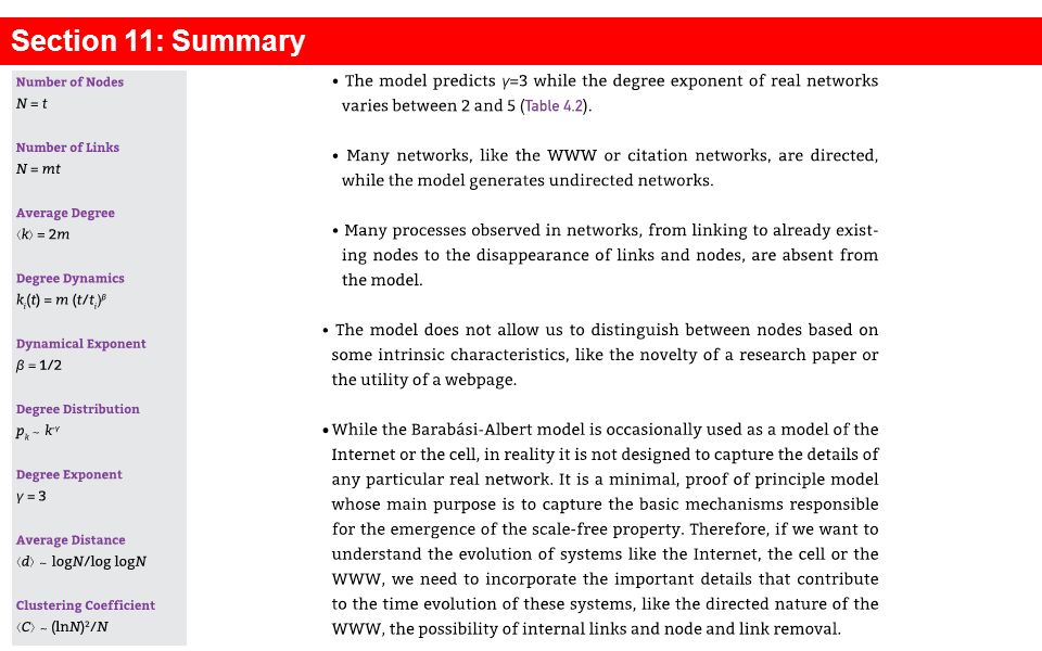
39. Nr. of nodes: Nr. of links: Average degree: Degree dynamics Degree distribution: Average Path Length: Clustering Coefficient: The network grows, but the degree distribution is stationary. β: dynamical exponent γ: degree exponent SUMMARY: PROPERTIES OF THE BA MODEL Network Science: Evolving Network Models February 2015

40. γ=1γ=2γ=3 diverges finite γ w in γ w out γ intern γ actor γ collab γ metab γ cita γ synonyms γ sex BA model Can we change the degree exponent? DEGREE EXPONENTS Network Science: Evolving Network Models February 2015

41. Evolving network models Network Science: Evolving Network Models February 2015

42. The BA model is only a minimal model. Makes the simplest assumptions: linear growth linear preferential attachment Does not capture variations in the shape of the degree distribution variations in the degree exponent the size-independent clustering coefficient Hypothesis: The BA model can be adapted to describe most features of real networks. We need to incorporate mechanisms that are known to take place in real networks: addition of links without new nodes, link rewiring, link removal; node removal, constraints or optimization EVOLVING NETWORK MODELS Network Science: Evolving Network Models February 2015

43. (the simplest way to change the degree exponent) Undirected BA network: Directed BA network: β=1: dynamical exponentγ in =2: degree exponent; P(k out )=δ(k out -m) Undirected BA: β=1/2; γ=3 BA ALGORITHM WITH DIRECTED EDGES Network Science: Evolving Network Models February 2015

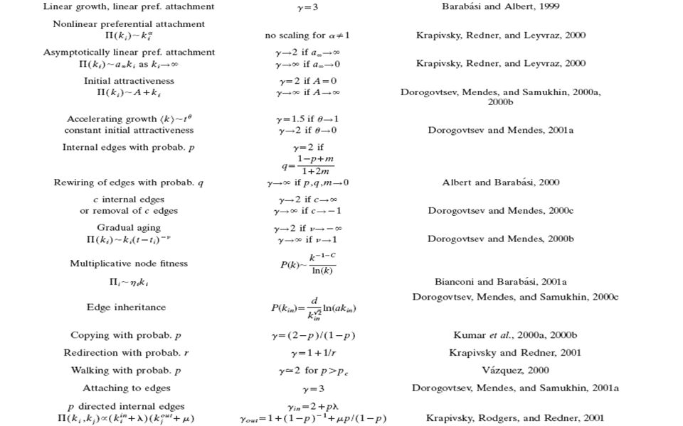
44. Extended Model prob. p : internal links prob. q : link deletion prob. 1-p-q : add node EXTENDED MODEL: Other ways to change the exponent P(k) ~ (k+  (p,q,m)) -  (p,q,m)   [1,  ) Network Science: Evolving Network Models February 2015

45. P(k) ~ (k+  (p,q,m)) -  (p,q,m)   [1,  ) Extended Model p=0.937 m=1  = 31.68  = 3.07 Actor network prob. p : internal links prob. q : link deletion prob. 1-p-q : add node  Predicts a small-k cutoff  a correct model should predict all aspects of the degree distribution, not only the degree exponent.  Degree exponent is a continuous function of p,q, m EXTENDED MODEL: Small-k cutoff Network Science: Evolving Network Models February 2015

46. Non-linear preferential attachment:  P(k) does not follow a power law for  1   <1 : stretch-exponential   >1 : no-scaling (  >2 : “gelation”) P. Krapivsky, S. Redner, F. Leyvraz, Phys. Rev. Lett. 85, 4629 (2000) NONLINEAR PREFERENTIAL ATTACHMENT: MORE MODELS Network Science: Evolving Network Models February 2015

47. Initial attractiveness shifts the degree exponent: A - initial attractiveness Dorogovtsev, Mendes, Samukhin, Phys. Rev. Lett. 85, 4633 (2000) BA model: k=0 nodes cannot aquire links, as Π(k=0)=0 (the probability that a new node will attach to it is zero) Note: the parameter A can be measured from real data, being the rate at which k=0 nodes acquire links, i.e. Π(k=0)=A INITIAL ATTRACTIVENESS Network Science: Evolving Network Models February 2015

48. Finite lifetime to acquire new edges Gradual aging: S. N. Dorogovtsev and J. F. F. Mendes, Phys. Rev. E 62, 1842 (2000) L. A. N. Amaral et al., PNAS 97, 11149 (2000) GROWTH CONSTRAINTS AND AGING CAUSE CUTOFFS Network Science: Evolving Network Models February 2015

49. P(k) ~ k -  Pathlenght Clustering Degree Distr. P(k)=δ(k-k d ) Exponential P(k) ~ k -  THE LAST PROBLEM: HIGH, SYSTEM-SIZE INDEPENDENT C(N) Regular network Erdos- Renyi Watts- Strogatz Barabasi- Albert Network Science: Evolving Network Models February 2015

50. Each node of the network can be either active or inactive. There are m active nodes in the network in any moment. 1.Start with m active, completely connected nodes. 2.Each timestep add a new node (active) that connects to m active nodes. 3.Deactivate one active node with probability: K. Klemm and V. Eguiluz, Phys. Rev. E 65, 036123 (2002) C  C* when N  ∞ A MODEL WITH HIGH CLUSTERING COEFFICIENT Network Science: Evolving Network Models February 2015

52. Fitness Model Network Science: Evolving Network Models February 2015

53. SF model: k(t)~t ½ (first mover advantage) Fitness model: fitness (  k( ,t)~t   =  C Fitness Model: Can Latecomers Make It? time Degree (k) Bianconi & Barabási, Physical Review Letters 2001; Europhys. Lett. 2001.

54. Bose-Einstein condensation Fit-gets-rich FITNESS MODEL: Can Latecomers Make It?

55. The network grows, but the degree distribution is stationary. Section 11: Summary

56. The network grows, but the degree distribution is stationary. Section 11: Summary

58. 1. There is no universal exponent characterizing all networks. 2.Growth and preferential attachment are responsible for the emergence of the scale-free property. 3.The origins of the preferential attachment is system-dependent. 4. Modeling real networks: identify the microscopic processes that take place in the system measure their frequency from real data develop dynamical models that capture these processes. 5. If the model is correct, it should correctly predict not only the degree exponent, but both small and large k-cutoffs. LESSONS LEARNED: evolving network models Network Science: Evolving Network Models February 2015

59. Philosophical change in network modeling: ER, WS models are static models – the role of the network modeler it to cleverly place the links between a fixed number of nodes to that the network topology mimic the networks seen in real systems. BA and evolving network models are dynamical models: they aim to reproduce how the network was built and evolved. Thus their goal is to capture the network dynamics, not the structure.  as a byproduct, you get the topology correctly LESSONS LEARNED: evolving network models Network Science: Evolving Network Models February 2015

60. The end Network Science: Evolving Network Models February 2015