1. Albert-László Barabási
Network Science
Class 5: BA model
(Sept 15, 2014)
Albert-László Barabási
With
Roberta Sinatra
We all have our theories of the origin of this mess. And we may also differ in the way we would like to see the solutions. But we all agree on one thing– it is the incerconnectedness of the system that is at the heart to wash away the problem with a single instruction.

2. Section 1
Introduction

3. Section 1
Hubs represent the most striking difference between a random and a scale-free network. Their emergence in many real systems raises several fundamental questions:
Why does the random network model of Erdős and Rényi fail to reproduce the hubs and the power laws observed in many real networks?
Why do so different systems as the WWW or the cell converge to a similar scale-free architecture?
he last question is particularly puzzling given the fundamental differences in the nature, origin, and scope of the systems that display the scale-free property:
The nodes of the cellular network are proteins or metabolites, while the nodes of the WWW are documents, representing information without a physical manifestation.
The links within the cell are binding interactions and chemical reactions, while the links of the WWW are URLs, or small segments of computer code.
The history of these two systems could not be more different: the cellular network is shaped by 4 billion years of evolution, while the WWW is only a few decades old.
The purpose of the metabolic network is to produce the basic chemical components the cells need to survive, while the purpose of the WWW is information access and delivery.
To understand why so different systems converge to a similar architecture we need to first uncover the mechanism responsible for the emergence of the scale-free property. This is the main topic of this chapter. Given the major differences between the systems that display the scale-free property, the explanation must be simple and fundamental. The answers will change the way we view and model networks, forcing us to move from describing a network’s topology to modeling the evolution of complex systems.

4. Growth and preferential attachment
Section 2
Growth and preferential attachment

5. networks expand through the addition of new nodes
BA model: Growth
BA MODEL: Growth
ER model:
the number of nodes, N, is fixed (static models)
networks expand through the addition of new nodes
Barabási & Albert, Science 286, 509 (1999)

6. New nodes prefer to connect to the more connected nodes
BA model: Growth
BA MODEL: Preferential attachment
ER model: links are added randomly to the network
New nodes prefer to connect to the more connected nodes
We are familiar with only a tiny fraction of the trillion or more documents available on the WWW. The nodes we know are not entirely random: we all heard about Google and Facebook, but we rarely encounter the billions of less-prominent nodes that populate the Web. As our knowledge is biased towards the more connected nodes, we are more likely to link to a hub than to a node with only few links.
With more than a million scientific papers published each year, no scientist can attempt to read them all. The more cited is a paper, the more likely that we will notice it. Therefore, our citations are biased towards the more cited publications, representing the high-degree nodes of the citation network.
The more movies an actor has played in, the more familiar is a casting director with her skills. Hence, the higher the degree of an actor in the actor network, the higher are the chances that he/she will be considered for a new role.
Barabási & Albert, Science 286, 509 (1999)
Network Science: Evolving Network Models February 14, 2011

7. BA model: Growth Section 2: Growth and Preferential Sttachment
The random network model differs from real networks in two important characteristics:
Growth: While the random network model assumes that the number of nodes is fixed (time invariant), real networks are the result of a growth process that continuously increases.
Preferential Attachment: While nodes in random networks randomly choose their interaction partner, in real networks new nodes prefer to link to the more connected nodes.
Barabási & Albert, Science 286, 509 (1999)
Network Science: Evolving Network Models February 14, 2011

8. The Barabási-Albert model
Section 3
The Barabási-Albert model

9. Origin of SF networks: Growth and preferential attachment
(1) Networks continuously expand by the addition of new nodes
WWW : addition of new documents
GROWTH:
add a new node with m links
PREFERENTIAL ATTACHMENT:
the probability that a node connects to a node with k links is proportional to k.
(2) New nodes prefer to link to highly connected nodes.
WWW : linking to well known sites
P(k) ~k-3
Barabási & Albert, Science 286, 509 (1999)
Network Science: Evolving Network Models February 14, 2011

10. Section 4
The degree distribution of a network generated by the Barabási-Albert model. The plot show for a single network of size N=100,000 and m=3 and . It shows both the linearly-binned (red symbols) as well as the log-binned version (green symbols) o. The straight line is added to guide the eye and has slope -3, corresponding to the resulting network’s degree exponent.

11. The discovery of the Barabási-Albert model is recounted in Linked [9], describing a workstop in Porto, Portugal, attended by the first author of the model: “During the summer of 1999 very few people were thinking about networks, and there were no talks on the subject during this workshop. But networks were very much on my mind. I could not help carrying with me on the trip our unresolved questions: Why hubs? Why power-laws? […] Before I left for Europe, Réka Albert and I agreed that she would analyze these networks. On June 14, a week after my departure, I received a long from her detailing some ongoing activities. At the end of the message there was a sentence added like an afterthought: “I looked at the connectivity distribution too, and in almost all systems (IBM, actors, power grid), the tail of the distribution follows a power law.”
Réka’s suddenly made it clear that the Web was by no means special. I found myself sitting in the conference hall paying no attention to the talks, thinking about the implications of this finding. If two networks as different as the Web and the Hollywood acting community both display power-law degree distribution, then some universal law or mechanism must be responsible. If such a law existed, it could potentially apply to all networks.
During the first break between talks I decided to withdraw to the quiet of the seminary where we were housed during the workshop. I did not get far, however. During the fifteen-minute walk back to my room a potential explanation occurred to me, one so simple and straightforward that I doubted it could be right. I immediately returned to the university to fax Réka, asking her to verify the idea using the computer. A few hours later she ed me the answer. To my great astonishment, the idea worked.”
The two images above reproduce the fax sent on June 14, 1999 from Porto, describing the algorithm that we call today the Barabási-Albert model.

12. Section 4 Linearized Chord Diagram

13. Section 4
Degree dynamics

14. All nodes follow the same growth law
Use:
During a unit time (time step): Δk=m  A=m
This is an important prediction, as it implies that all nodes follow the same growth law. Hence the difference between the hubs is not in the fact that hubs grow faster, but that they are older. Indeed, the difference between the nodes comes in the intercept of the power-law, controlled by $t_i$, representing the time at which node $i$ joined the network.
If all nodes follow the same growth rate, why do we have hubs and less connected nodes in the network? The reason is that at moment older nodes have a higher degree according to Eq. \ref{connect}--indeed, the smaller $t_i$ is, the higher is the node's degree. As a consequence older nodes acquire more links in an unit time. This is seen by inspective the derivative of Eq. \ref{connect}, which is nothing but the node's growth rate (i.e. the rate at which the node acquires new links)
with predicts two things. First, it tells is that the older the node is (i.e. the smaller $t_i$ is), the larger the growth rate. Second, it also tells us that with time the rate at which the nodes acquire links goes down, thanks to the fact that the new nodes have many more nodes to link to.
β: dynamical exponent
A.-L.Barabási, R. Albert and H. Jeong, Physica A 272, 173 (1999)
Network Science: Evolving Network Models February 14, 2011

15. SF model: k(t)~t ½ (first mover advantage)
All nodes follow the same growth law
SF model: k(t)~t ½ (first mover advantage)
Degree (k)
This is an important prediction, as it implies that all nodes follow the same growth law. Hence the difference between the hubs is not in the fact that hubs grow faster, but that they are older. Indeed, the difference between the nodes comes in the intercept of the power-law, controlled by $t_i$, representing the time at which node $i$ joined the network.
If all nodes follow the same growth rate, why do we have hubs and less connected nodes in the network? The reason is that at moment older nodes have a higher degree according to Eq. \ref{connect}--indeed, the smaller $t_i$ is, the higher is the node's degree. As a consequence older nodes acquire more links in an unit time. This is seen by inspective the derivative of Eq. \ref{connect}, which is nothing but the node's growth rate (i.e. the rate at which the node acquires new links)
with predicts two things. First, it tells is that the older the node is (i.e. the smaller $t_i$ is), the larger the growth rate. Second, it also tells us that with time the rate at which the nodes acquire links goes down, thanks to the fact that the new nodes have many more nodes to link to.
time

16. Section 5.3

17. Section 5
Degree distribution

18. γ = 3 Degree distribution
A node i can come with equal probability any time between ti=m0 and t, hence:
γ = 3
PREDICTIONS:
(i) The degree exponent $\gamma$ is independent of $m$, a prediction that is in agreement with the numerical results (see Fig. 4).
(ii) As the power-law observed for real networks describes systems of rather different ages and sizes, it is expected that a correct model should provide a time-independent degree distribution. Indeed, Eq.(\ref{cube}) predicts that asymptotically (i.e. in the $t \gg m_0$ limit) the degree distribution of the BA model is independent of time (and, subsequently, independent of the system size $N=m_0+t$), indicating that despite its continuous growth, the network reaches a stationary scale-free state.
Nominal similarities shown in Figure 4 support these predictions.
(iii) Equation (\ref{cube}) indicates that the coefficient of the power-law distribution is proportional to $m^2$. a prediction again confirmed by the numerical simulations shown in Figure \ref{F-BA-BAScaling}.
A.-L.Barabási, R. Albert and H. Jeong, Physica A 272, 173 (1999)
Network Science: Evolving Network Models February 14, 2011

19. γ = 3 Degree distribution (i) The degree exponent is independent of m.
(ii) As the power-law describes systems of rather different ages and sizes, it is expected that a correct model should provide a time-independent degree distribution. Indeed, asymptotically the degree distribution of the BA model is independent of time (and of the system size N)
 the network reaches a stationary scale-free state.
(iii) The coefficient of the power-law distribution is proportional to m2.
PREDICTIONS:
(i) The degree exponent $\gamma$ is independent of $m$, a prediction that is in agreement with the numerical results (see Fig. 4).
(ii) As the power-law observed for real networks describes systems of rather different ages and sizes, it is expected that a correct model should provide a time-independent degree distribution. Indeed, Eq.(\ref{cube}) predicts that asymptotically (i.e. in the $t \gg m_0$ limit) the degree distribution of the BA model is independent of time (and, subsequently, independent of the system size $N=m_0+t$), indicating that despite its continuous growth, the network reaches a stationary scale-free state.
Nominal similarities shown in Figure 4 support these predictions.
(iii) Equation (\ref{cube}) indicates that the coefficient of the power-law distribution is proportional to $m^2$. a prediction again confirmed by the numerical simulations shown in Figure \ref{F-BA-BAScaling}.
A.-L.Barabási, R. Albert and H. Jeong, Physica A 272, 173 (1999)
Network Science: Evolving Network Models February 14, 2011

20. The mean field theory offers the correct scaling, BUT it provides the wrong coefficient of the degree distribution. So assymptotically it is correct (k ∞), but not correct in details (particularly for small k). To fix it, we need to calculate P(k) exactly, which we will do next using a rate equation based approach.
Network Science: Evolving Network Models February 14, 2011

21. MFT - Degree Distribution: Rate Equation
Number of nodes with degree k at time t.
Since at each timestep we add one node, we have N=t (total number of nodes =number of timesteps)
2m: each node adds m links, but each link contributed to the degree of 2 nodes
Total number of k-nodes
Number of links added to degree k nodes after the arrival of a new node:
Nr. of degree k-1 nodes that acquire a new link, becoming degree k
New node adds m new links to other nodes
Preferential attachment
Nr. of degree k nodes that acquire a new link, becoming degree k+1
Loss of k-nodes via
k k+1
# k-nodes at time t+1
# k-nodes at time t
Gain of k-nodes via
k-1 k

22. MFT - Degree Distribution: Rate Equation
Gain of k-nodes via
k-1 k
Loss of k-nodes via
k k+1
# k-nodes at time t+1
# k-nodes at time t
We do not have k=0,1,...,m-1 nodes in the network (each node arrives with degree m)
 We need a separate equation for degree m modes
# m-nodes at time t+1
# m-nodes at time t
Add one
m-degeree node
Loss of an
m-node via
m m+1
Network Science: Evolving Network Models February 14, 2011
A.-L.Barabási, R. Albert and H. Jeong, Physica A 272, 173 (1999)

23. MFT - Degree Distribution: Rate Equation
k>m
We assume that there is a stationary state in the N=t∞ limit, when P(k,∞)=P(k)
k>m
Network Science: Evolving Network Models February 14, 2011
A.-L.Barabási, R. Albert and H. Jeong, Physica A 272, 173 (1999)

24. ... MFT - Degree Distribution: Rate Equation 
m+3  k
...
for large k
Krapivsky, Redner, Leyvraz, PRL 2000
Dorogovtsev, Mendes, Samukhin, PRL 2000
Bollobas et al, Random Struc. Alg. 2001
Network Science: Evolving Network Models February 14, 2011
A.-L.Barabási, R. Albert and H. Jeong, Physica A 272, 173 (1999)

25. MFT - Degree Distribution: A Pretty Caveat
Start from eq.
Its solution is:
Dorogovtsev and Mendes, 2003
Network Science: Evolving Network Models February 14, 2011
A.-L.Barabási, R. Albert and H. Jeong, Physica A 272, 173 (1999)

26. γ = 3 Degree distribution (i) The degree exponent is independent of m.
for large k
(i) The degree exponent is independent of m.
(ii) As the power-law describes systems of rather different ages and sizes, it is expected that a correct model should provide a time-independent degree distribution. Indeed, asymptotically the degree distribution of the BA model is independent of time (and of the system size N)
 the network reaches a stationary scale-free state.
(iii) The coefficient of the power-law distribution is proportional to m2.
PREDICTIONS:
(i) The degree exponent $\gamma$ is independent of $m$, a prediction that is in agreement with the numerical results (see Fig. 4).
(ii) As the power-law observed for real networks describes systems of rather different ages and sizes, it is expected that a correct model should provide a time-independent degree distribution. Indeed, Eq.(\ref{cube}) predicts that asymptotically (i.e. in the $t \gg m_0$ limit) the degree distribution of the BA model is independent of time (and, subsequently, independent of the system size $N=m_0+t$), indicating that despite its continuous growth, the network reaches a stationary scale-free state.
Nominal similarities shown in Figure 4 support these predictions.
(iii) Equation (\ref{cube}) indicates that the coefficient of the power-law distribution is proportional to $m^2$. a prediction again confirmed by the numerical simulations shown in Figure \ref{F-BA-BAScaling}.
Network Science: Evolving Network Models February 14, 2011

27. NUMERICAL SIMULATION OF THE BA MODEL

28. absence of growth and preferential attachment
Section 6
absence of growth and preferential attachment

29. MODEL A
growth preferential attachment
Π(ki) : uniform

30. pk : power law (initially)   Gaussian  Fully Connected
MODEL B
growth preferential attachment
pk : power law (initially) 
 Gaussian  Fully Connected

31. Do we need both growth and preferential attachment? YEP.
Network Science: Evolving Network Models February 14, 2011

32. Measuring preferential attachment
Section 7
Measuring preferential attachment

33. Section 7 Measuring preferential attachment
Plot the change in the degree Δk during
a fixed time Δt for nodes with degree k.
To reduce noise, plot the integral of Π(k) over k:
No pref. attach:
κ~k
Linear pref. attach: κ~k2
(Jeong, Neda, A.-L. B, Europhys Letter 2003; cond-mat/ )
Network Science: Evolving Network Models February 14, 2011

34. Plots shows the integral of Π(k) over k:
Section 7 Measuring preferential attachment
citation network
Plots shows the integral of Π(k) over k:
Internet
No pref. attach:
κ~k
actor collab.
neurosci collab
Linear pref. attach: κ~k2
Network Science: Evolving Network Models February 14, 2011

35. Nonlinear preferenatial attachment
Section 8
Nonlinear preferenatial attachment

36. Section 8 Nonlinear preferential attachment
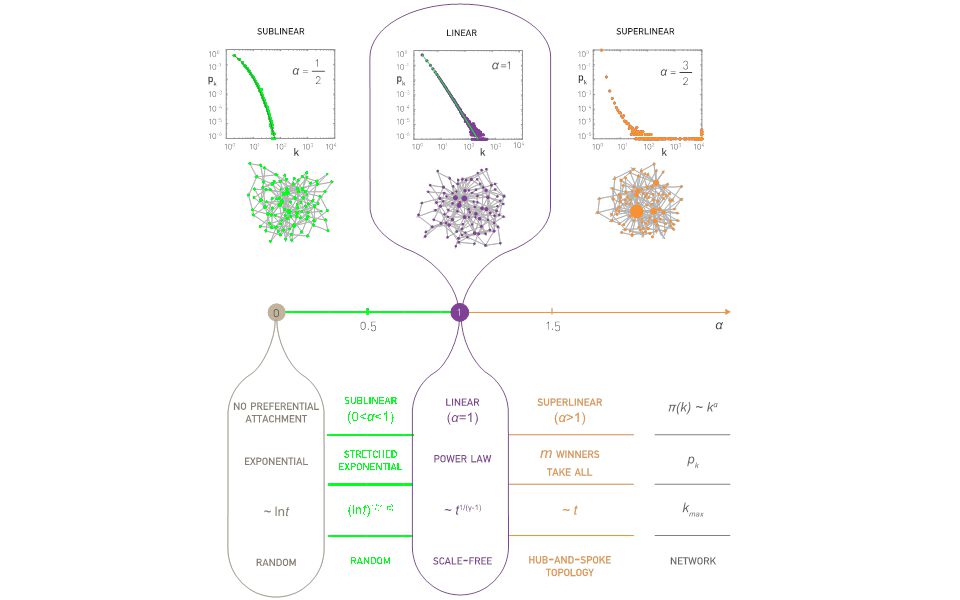
α=0: Reduces to Model A discussed in Section 5.4. The degree distribution follows the simple exponential function.
α=1: Barabási-Albert model, a scale-free network with degree exponent 3.
0<α<1: Sublinear preferential attachment. New nodes favor the more connected nodes over the less connected nodes. Yet, for the bias is not sufficient to generate a scale-free degree distribution. Instead, in this regime the degrees follow the stretched exponential distribution:

37. Section 8 Nonlinear preferential attachment
α=0: Reduces to Model A discussed in Section 5.4. The degree distribution follows the simple exponential function.
α=1: Barabási-Albert model, a scale-free network with degree exponent 3.
α>1: Superlinear preferential attachment. The tendency to link to highly connected nodes is enhanced, accelerating the “rich-gets-richer” process. The consequence of this is most obvious for , when the model predicts a winner-takes-all phenomenon: almost all nodes connect to a single or a few super-hubs.

38. Section 8 Nonlinear preferential attachment
The growth of the hubs. The nature of preferential attachment affects the degree of the largest node. While in a scale-free network the biggest hub grows as (green curve), for sublinear preferential attachment this dependence becomes logarithmic (red curve). For superlinear preferential attachment the biggest hub grows linearly with time, always grabbing a finite fraction of all links (blue curve)). The symbols are provided by a numerical simulation; the dotted lines represent the analytical predictions.

40. The origins of preferential attachment
Section 9
The origins of preferential attachment
Given the important role preferential attachment plays in the evolution of real networks, we must ask: where does preferential attachment come from? Specifically,
Why does depend on ?
Why is the dependence of linear in k ?
There are two philosophically different takes on these questions. The first approach views preferential attachment as an interplay between random events and some structural network property. These mechanisms do not require global knowledge of the network. Hence we will call them local or random mechanisms. The second approach assumes that the addition of each new node or link is preceeded by a cost-benefit analysis, balancing various needs with the available resources. This assumes familiarity with the whole network and relies on optimization principles, prompting us to call them global or optimized mechanisms. The purpose of this section is to discuss these two approaches.

41. Section 9 Link selection model
Link selection model -- perhaps the simplest example of a local or random mechanism capable of generating preferential attachment.
Growth: at each time step we add a new node to the network.
Link selection: we select a link at random and connect the new node to one of nodes at the two ends of the selected link.
To show that this simple mechanism generates linear preferential attachment, we write the probability that the node at the end of a randomly chosen link has degree k as

42. Section 9 Copying model

(a) Random Connection: with probability p the new node links to u.

(b) Copying: with probability we randomly choose an outgoing link of node u and connect the new node to the selected link's target. Hence the new node “copies” one of the links of an earlier node
(a) the probability of selecting a node is 1/N.
(b) is equivalent with selecting a node linked to a randomly selected link. The probability of selecting a degree-k node through the copying process of step (b) is k/2L for undirected networks.
The likelihood that the new node will connect to a degree-k node follows preferential attachment
Social networks: Copy your friend’s friends.
Citation Networks: Copy references from papers we read.
Protein interaction networks: gene duplication,
When building a new webpage, authors tend to borrow links from webpages covering similar topics, a process captured by the copying model [17, 18]. In the model in each time step a new node with a single link is added to the network. To choose the target node we randomly select a node u and follow a two-step procedure:

43. Section 9 Optimization model
A longstanding assumption of economics is that humans make rational decisions, balancing cost against benefits. In other words, each individual aims to maximize its personal advantage. This is the starting point of rational choice theory in economics [21] and it is a hypothesis central to modern political science, sociology and philosophy. As we show below, such rational decisions can lead to preferential attachment [22, 23, 24].
Consider the Internet, whose nodes are routers connected via cables. Establishing a new Internet connection between two routers requires us to lay down a new cable between them. As this is costly, each new link is preceded by a careful cost-benefit analysis. Each new router (node) will choose its link to balance access to good network performance (i.e. proper bandwith) with the cost of laying down a new cable (i.e. physical distance). This can be a conflicting desire, as the closest node may not offer the best network performance.

44. Section 9 Optimization model

45. Section 9 Optimization model

46. Section 9 Optimization model

47. Section 9
Given the important role preferential attachment plays in the evolution of real networks, we must ask: where does preferential attachment come from? Specifically,
Why does depend on ?
Why is the dependence of linear in k ?
There are two philosophically different takes on these questions. The first approach views preferential attachment as an interplay between random events and some structural network property. These mechanisms do not require global knowledge of the network. Hence we will call them local or random mechanisms. The second approach assumes that the addition of each new node or link is preceeded by a cost-benefit analysis, balancing various needs with the available resources. This assumes familiarity with the whole network and relies on optimization principles, prompting us to call them global or optimized mechanisms. The purpose of this section is to discuss these two approaches.

48. Diameter and clustering coefficient
Section 10
Diameter and clustering coefficient

49. Section Diameter
Bollobas, Riordan, 2002

50. Section 10 Clustering coefficient
Reminder: for a random graph we have:
What is the functional form of C(N)?
Konstantin Klemm, Victor M. Eguiluz,
Growing scale-free networks with small-world behavior,
Phys. Rev. E 65, (2002), cond-mat/

51. CLUSTERING COEFFICIENT OF THE BA MODEL1 2
Denote the probability to have a link between node i and j with P(i,j)
The probability that three nodes i,j,l form a triangle is P(i,j)P(i,l)P(j,l)
The expected number of triangles in which a node l with degree kl participates is thus:
We need to calculate P(i,j).
Network Science: Evolving Network Models February 14, 2011

52. CLUSTERING COEFFICIENT OF THE BA MODEL
Calculate P(i,j).
Node j arrives at time tj=j and the probability that it will link to node i with degree ki already in the network is determined by preferential attachment:
Where we used that the arrival time of node j is tj=j and the arrival time of node is ti=i
Which is the degree of node l at current time, at time t=N
Let us approximate:
There is a factor of two difference... Where does it come from?
Network Science: Evolving Network Models February 14, 2011

53. Section 10 Clustering coefficient
Reminder: for a random graph we have:
What is the functional form of C(N)?
Konstantin Klemm, Victor M. Eguiluz,
Growing scale-free networks with small-world behavior,
Phys. Rev. E 65, (2002), cond-mat/

54. Section 11: Summary
The network grows, but the degree distribution is stationary.

55. Section 11: Summary
The network grows, but the degree distribution is stationary.

56. Section 11: Summary