Download presentation
Presentation is loading. Please wait.

1
Recognition (classification) = assigning a pattern/object to one of pre-defined classes Statictical (feature-based) PR - the pattern is described by features (n-D vector in a metric space) Pattern Recognition
 = assigning a pattern/object to one of pre-defined classes Statictical (feature-based) PR - the pattern is described by features (n-D vector in a metric space) Pattern Recognition")
2
Recognition (classification) = assigning a pattern/object to one of pre-defined classes Syntactic (structural) PR - the pattern is described by its structure. Formal language theory (class = language, pattern = word) Pattern Recognition
 Pattern Recognition.")
3
Supervised PR – training set available for each class Unsupervised PR (clustering) – training set not available, No. of classes may not be known Pattern Recognition

4
PR system - Training stage Definition of the features Selection of the training set Computing the features of the training set Classification rule setup

5
Desirable properties of the features Invariance Discriminability Robustness Efficiency, independence, completeness

6
Desirable properties of the training set It should contain typical representatives of each class including intra-class variations Reliable and large enough Should be selected by domain experts

7
Classification rule setup Equivalent to a partitioning of the feature space Independent of the particular application

8
PR system – Recognition stage Image acquisition Preprocessing Object detection Computing of the features Classification Class label

9
An example – Fish classification

10
The features: Length, width, brightness

11
2-D feature space

12
Empirical observation For a given training set, we can have several classifiers (several partitioning of the feature space) The training samples are not always classified correctly We should avoid overtraining of the classifier
 The training samples are not always classified correctly We should avoid overtraining of the classifier")
13
Formal definition of the classifier Each class is characterized by its discriminant function g(x) Classification = maximization of g(x) Assign x to class i iff Discriminant functions defines decision boundaries in the feature space
 Classification = maximization of g(x) Assign x to class i iff Discriminant functions defines decision boundaries in the feature space")
14
Minimum distance (NN) classifier Discriminant function g(x) = 1/ dist(x, ) Various definitions of dist(x One-element training set
 classifier Discriminant function g(x) = 1/ dist(x, ) Various definitions of dist(x One-element training set ")
15
Voronoi polygons

16
Minimum distance (NN) classifier Discriminant function g(x) = 1/ dist(x, ) Various definitions of dist(x One-element training set Voronoi pol NN classifier may not be linear NN classifier is sensitive to outliers k-NN classifier
 classifier Discriminant function g(x) = 1/ dist(x, ) Various definitions of dist(x One-element training set Voronoi pol NN classifier may not be linear NN classifier is sensitive to outliers k-NN classifier")
17
Find nearest training points unless k samples belonging to one class is reached

18
Discriminant functions g(x) are hyperplanes Linear classifier
 are hyperplanes Linear classifier")
19
Assumption: feature values are random variables Statistic classifier, the decission is probabilistic It is based on the Bayes rule Bayesian classifier

20
The Bayes rule A posteriori probability Class-conditional probability A priori probability Total probability

21
Bayesian classifier Main idea: maximize posterior probability Since it is hard to do directly, we rather maximize In case of equal priors, we maximize only

22
Equivalent formulation in terms of discriminat functions

23
How to estimate ? Parametric estimate (assuming pdf is of known form, e.g. Gaussian) Non-parametric estimate (pdf is unknown or too complex) From the case studies performed before (OCR, speech recognition) From the occurence in the training set Assumption of equal priors
 Non-parametric estimate (pdf is unknown or too complex) From the case studies performed before (OCR, speech recognition) From the occurence in the training set Assumption of equal priors.")
24
Parametric estimate of Gaussian

25
d-dimensional Gaussian pdf

26
The role of covariance matrix

27
Two-class Gaussian case in 2D Classification = comparison of two Gaussians

28
Two-class Gaussian case – Equal cov. mat. Linear decision boundary

29
Equal priors Classification by minimum Mahalanobis distance If the cov. mat. is diagonal with equal variances then we get “standard” minimum distance rule max min

30
Non-equal priors Linear decision boundary still preserved

31
General G case in 2D Decision boundary is a hyperquadric

32
General G case in 3D Decision boundary is a hyperquadric

33
More classes, Gaussian case in 2D

34
What to do if the classes are not normally distributed? Gaussian mixtures Parametric estimation of some other pdf Non-parametric estimation

35
Non-parametric estimation – Parzen window

36
The role of the window size Small window overtaining Large window data smoothing Continuous data the size does not matter

37
n = 1 n = 10 n = 100 n = ∞

38
The role of the window size Small window Large window

39
Applications of Bayesian classifier in multispectral remote sensing Objects = pixels Features = pixel values in the spectral bands (from 4 to several hundreds) Training set – selected manually by means of thematic maps (GIS), and on-site observation Number of classes – typicaly from 2 to 16
 Training set – selected manually by means of thematic maps (GIS), and on-site observation Number of classes – typicaly from 2 to 16")
40
Satellite MS image

41
Other classification methods in RS Context-based classifiers Shape and textural features Post-classification filtering Spectral pixel unmixing

42
Typically for “YES – NO” features Feature metric is not explicitely defined Decision trees Non-metric classifiers

43
General decision tree

44
Binary decision tree Any decision tree can be replaced by a binary tree

45
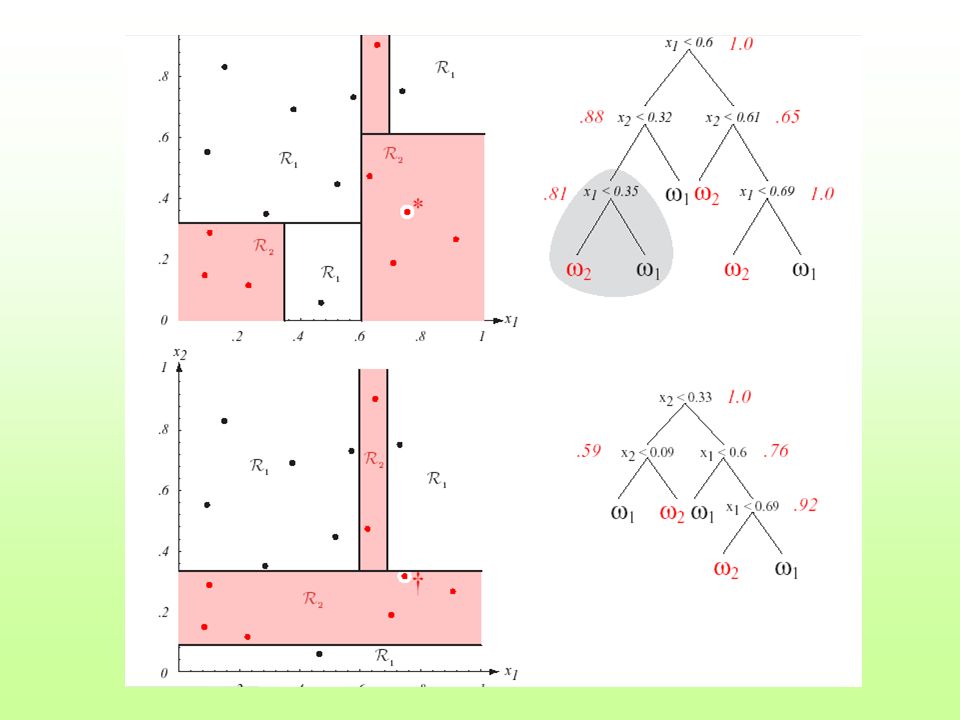
Real-valued features Node decisions are in form of inequalities Training = setting their parameters Simple inequalities stepwise decision boundary

46
Stepwise decision boundary

47
Real-valued features The tree structure and the form of inequalities influence both performance and speed.

50
How to evaluate the performance of the classifiers? - evaluation on the training set (optimistic error estimate) - evaluation on the test set (pesimistic error estimate) Classification performance
 - evaluation on the test set (pesimistic error estimate) Classification performance.")
51
How to increase the performance? - other features - more features (dangerous – curse of dimensionality!) - other (larger, better) traning sets - other parametric model - other classifier - combining different classifiers Classification performance
 - other (larger, better) traning sets - other parametric model - other classifier - combining different classifiers Classification performance.")
52
Combining (fusing) classifiers C feature vectors Bayes rule: max max Several possibilities how to do that
 classifiers C feature vectors Bayes rule: max max Several possibilities how to do that")
53
Product rule Assumption: Conditional independence of x j max

54
Max-max and max-min rules Assumption: Equal priors max (max ) max (min )
 max (min )")
55
Majority vote The most straightforward fusion method Can be used for all types of classifiers

56
Training set is not available, No. of classes may not be a priori known Unsupervised Classification (Cluster analysis)
.")
57
What are clusters? Intuitive meaning - compact, well-separated subsets Formal definition - any partition of the data into disjoint subsets

58
What are clusters?

59
How to compare different clusterings? Variance measure J should be minimized Drawback – only clusterings with the same N can be compared. Global minimum J = 0 is reached in the degenerated case.

60
Clustering techniques Iterative methods - typically if N is given Hierarchical methods - typically if N is unknown Other methods - sequential, graph-based, branch & bound, fuzzy, genetic, etc.

61
Sequential clustering N may be unknown Very fast but not very good Each point is considered only once Idea: a new point is either added to an existing cluster or it forms a new cluster. The decision is based on the user-defined distance threshold.

62
Sequential clustering Drawbacks: -Dependence on the distance threshold -Dependence on the order of data points

63
Iterative clustering methods N-means clustering Iterative minimization of J ISODATA Iterative Self-Organizing DATa Analysis

64
N-means clustering 1.Select N initial cluster centroids.

65
N-means clustering 2. Classify every point x according to minimum distance.

66
N-means clustering 3. Recalculate the cluster centroids.

67
N-means clustering 4. If the centroids did not change then STOP else GOTO 2.

68
N-means clustering Drawbacks - The result depends on the initialization. - J is not minimized - The results are sometimes “intuitively wrong”.

69
N-means clustering – An example Two features, four points, two clusters (N = 2) Different initializations different clusterings
 Different initializations different clusterings")
70
Initial centroids N-means clustering – An example

71
Initial centroids N-means clustering – An example

72
Iterative minimization of J 1.Let’s have an initial clustering (by N-means) 2.For every point x do the following: Move x from its current cluster to another cluster, such that the decrease of J is maximized. 3. If all data points do not move, then STOP.

73
Example of “wrong” result

74
ISODATA Iterative clustering, N may vary. Sophisticated method, a part of many statistical software systems. Postprocessing after each iteration -Clusters with few elements are cancelled -Clusters with big variance are divided -Other merging and splitting strategies can be implemented

75
Hierarchical clustering methods Agglomerative clustering Divisive clustering

76
Basic agglomerative clustering 1.Each point = one cluster

77
Basic agglomerative clustering 1.Each point = one cluster 2.Find two “nearest” or “most similar” clusters and merge them together

78
Basic agglomerative clustering 1.Each point = one cluster 2.Find two “nearest” or “most similar” clusters and merge them together 3.Repeat 2 until the stop constraint is reached

79
Basic agglomerative clustering Particular implementations of this method differ from each other by - The STOP constraints - The distance/similarity measures used

80
Simple between-cluster distance measures d(A,B) = d(m 1,m 2 ) d(A,B) = min d(a,b) d(A,B) = max d(a,b)
 = d(m 1,m 2 ) d(A,B) = min d(a,b) d(A,B) = max d(a,b)")
81
Other between-cluster distance measures d(A,B) = Hausdorf distance H(A,B) d(A,B) = J(AUB) – J(A,B)
 = Hausdorf distance H(A,B) d(A,B) = J(AUB) – J(A,B)")
82
Agglomerative clustering – representation by a clustering tree (dendrogram)
")
83
How many clusters are there? 2 or 4 ? Clustering is a very subjective task

84
How many clusters are there? Difficult to answer even for humans “Clustering tendency” Hierarchical methods – N can be estimated from the complete dendrogram The methods minimizing a cost function – N can be estimated from “knees” in J-N graph

85
Life time of the clusters Optimal number of clusters = 4

86
Optimal number of clusters

87
Applications of clustering in image proc. Segmentation – clustering in color space Preliminary classification of multispectral images Clustering in parametric space – RANSAC, image registration and matching Numerous applications are outside image processing area

88
References Duda, Hart, Stork: Pattern Clasification, 2 nd ed., Wiley Interscience, 2001 Theodoridis, Koutrombas: Pattern Recognition, 2 nd ed., Elsevier, 2003

Similar presentations


 and the class- conditional probabilities P(x|wi)>")
 by R. O. Duda, P. E. Hart and D. G. Stork, John.>")


 Vipin Kumar Army High Performance.>")
 by R. O. Duda, P. E. Hart and D. G. Stork, John.>")


 Ke Chen COMP24111 Machine Learning Revision slides are going to summarise all you have learnt from Part II, which should be helpful.>")
 by R. O. Duda, P. E. Hart and D. G. Stork, John Wiley.>")
>")

