Download presentation
Presentation is loading. Please wait.

1
ECONOMICS: Principles and Applications 3e HALL & LIEBERMAN © 2005 Thomson Business and Professional Publishing The Short-Run Macro Model

2
Figure 1 U.S. Consumption and Disposable Income, 1985–2002 2000 1995 1990 1985 Real Consumption Spending ($ Billions) 5,000 6,000 4,000 3,000 7,000 Real Disposable Income ($ Billions) 3,0004,0005,0006,0007,000
 5,000 6,000 4,000 3,000 7,000 Real Disposable Income ($ Billions) 3,0004,0005,0006,0007,000.")
3
Table 1 Hypothetical Data on Disposable Income and Consumption

4
Figure 2 The Consumption Function Consumption Function 1,000 600 The consumption function shows the (linear) relationship between real consumption spending and real disposable income and the slope of the line (0.6) is the marginal propensity to consume. Real Consumption Spending ($ Billions) 1,000 2,000 3,000 4,000 5,000 6,000 7,000 8,000 Real Disposable Income ($ Billions) 1,0002,0003,0004,0005,0006,0007,0008,000 The vertical intercept ($2,000 billion) is autonomous consumption spending...
 1,000 2,000 3,000 4,000 5,000 6,000 7,000 8,000 Real Disposable Income ($ Billions) 1,0002,0003,0004,0005,0006,0007,0008,000 The vertical intercept ($2,000 billion) is autonomous consumption spending....")
5
Table 2 The Relationship Between Consumption and Income

6
Figure 3 The Consumption– Income Line 1.To draw the consumption- income line, we measure real income (instead of real disposable income) on the horizontal axis. Consumption- Income Line 600 A B Real Consumption Spending ($ Billions) 1,000 2,000 3,000 4,000 5,000 5,600 Real Income ($ Billions) 2,0004,0006,0008,000 1,000 2.The line has the same slope as the consumption function in Figure 2... 3.but a different vertical intercept.
 1,000 2,000 3,000 4,000 5,000 5,600 Real Income ($ Billions) 2,0004,0006,0008,000 1,000 2.The line has the same slope as the consumption function in Figure but a different vertical intercept..")
7
Figure 4 A Shift in the Consumption–Income Line Consumption-Income Line When Net Taxes = 500 Consumption-Income Line When Net Taxes = 2,000 Real Consumption Spending ($ Billions) 1,000 2,000 3,000 4,000 5,000 6,000 7,000 8,000 Real Income ($ Billions) 2,0004,0006,0008,000
 1,000 2,000 3,000 4,000 5,000 6,000 7,000 8,000 Real Income ($ Billions) 2,0004,0006,0008,000")
8
Table 3 Changes in Consumption Spending and the Consumption–Income Line

9
Table 4 The Relationship Between Income and Aggregate Expenditure

10
Figure 5 Deriving the Aggregate Expenditure Line C + I P + G C + I P + G + NX C + I P C 2.then add planned investment (I P )... 1.Start with the consumption- income line, 5.to get the aggregate expenditure line. 3.government purchases (G)...4.and net exports (NX)... Real Aggregate Expenditure ($ Billions) 1,000 2,000 3,000 4,000 5,000 6,000 7,000 8,000 Real GDP ($ Billions) 2,000 4,0006,0008,000
...4.and net exports (NX)... Real Aggregate Expenditure ($ Billions) 1,000 2,000 3,000 4,000 5,000 6,000 7,000 8,000 Real GDP ($ Billions) 2,000 4,0006,0008,000.")
11
Figure 6 Using a 45° to Translate Distances A B 45° 0 2.we can translate any horizontal distance (such as 0B)... 3.into an equal vertical distance (BA). 1.Using a 45-degree line...
. 1.Using a 45-degree line....")
12
Figure 7 Determining Equilibrium Real GDP A Aggregate Expenditure E K H J Aggregate Expenditure Total Output Increase in Inventories 45° Real Aggregate Expenditure ($ Billions) 1,000 2,000 3,000 4,000 5,000 6,000 7,000 8,000 9,000 Real GDP ($ Billions) 2,0004,0006,0008,000 Decrease in Inventories C + I P + G + NX Total Output 9,000
 1,000 2,000 3,000 4,000 5,000 6,000 7,000 8,000 9,000 Real GDP ($ Billions) 2,0004,0006,0008,000 Decrease in Inventories C + I P + G + NX Total Output 9,000")
13
Figure 8 Equilibrium GDP Can Be Less than Full-Employment GDP $6,000 $7,000 E F AE LOW 75 Million $7,000 100 Million A B Aggregate Production Function $6,000 and equilibrium employment is less than full employment. When the aggregate expenditure line is low... Full EmploymentPotential GDP cyclical unemployment = 25 million Aggregate Expenditure ($ Billions) Real GDP ($ Billions) Real GDP ($ Billions) Number of Workers 45° equilibrium output ($6,000) is less than potential output,
 Real GDP ($ Billions) Real GDP ($ Billions) Number of Workers 45° equilibrium output ($6,000) is less than potential output,.")
14
Figure 9 Equilibrium GDP Can Be Greater than Full-Employment GDP $8,000 H $7,000 B Potential GDP Aggregate Expenditure ($ Billions) Real GDP ($ Billions) AE HIGH Real GDP ($ Billions) Number of Workers Aggregate Production Function 100 Million Full Employment 135 Million When the aggregate expenditure line is high... and equilibrium employ- ment is greater than full employment. equilibrium output ($8,000) is greater than potential output, F E'
 is greater than potential output, F E .")
15
Table 5 Cumulative Increases in Spending When Investment Spending Increases by $1,000 Billion

16
Figure 10 The Effect of a Change in Investment Spending 1,600 1,960 2,176 2,306 2,500 1,000 Initial Rise in I P After Round 2 After Round 3 After Round 4 After Round 5 Increase in Annual GDP After All Rounds …

17
Figure 1 1 A Graphical View of the Multiplier F E $2,500 Billion Real GDP ($ Billions) 2,0004,0006,0008,000 Real Aggregate Expenditure ($ Billions) 1,000 2,000 3,000 4,000 5,000 6,000 7,000 8,000 9,000 45° AE 2 AE 1 Increase in Equilibrium GDP $1,000 9,000
 2,0004,0006,0008,000 Real Aggregate Expenditure ($ Billions) 1,000 2,000 3,000 4,000 5,000 6,000 7,000 8,000 9,000 45° AE 2 AE 1 Increase in Equilibrium GDP $1,000 9,000")
18
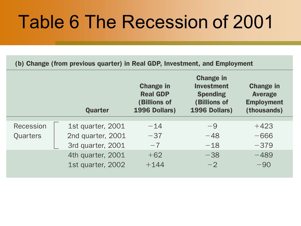
Table 6 The Recession of 2001

Similar presentations


>")
