1. Estuaries November 10

2. Flushing time (or residence time): time required to replace water with “new” water. Several ways to compute: Flushing time (or residence time): time required to replace water with “new” water. Several ways to compute: Tidal Prism method: Tidal Prism method: Where t f is number of tidal cycles required to “flush”; V is low tide volume of estuary V = (ave depth at MLLW) x (surface area) Assumes complete mixing of tidal prism volume with low tide volume – not very realistic: Can assume some mixing parameter α 0<α≤1: fraction of intertidal volume (tidal prism) mixed with low tide volume. But how do we determine α? In reality, water from head of estuary doesn’t get to mouth in 1 cycle; water that leaves on one cycle may return on next. One solution: Break estuary into segments each size of 1 tidal excursion

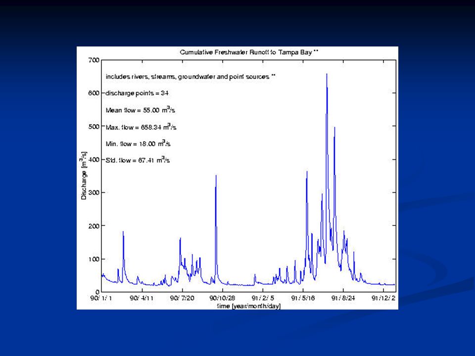
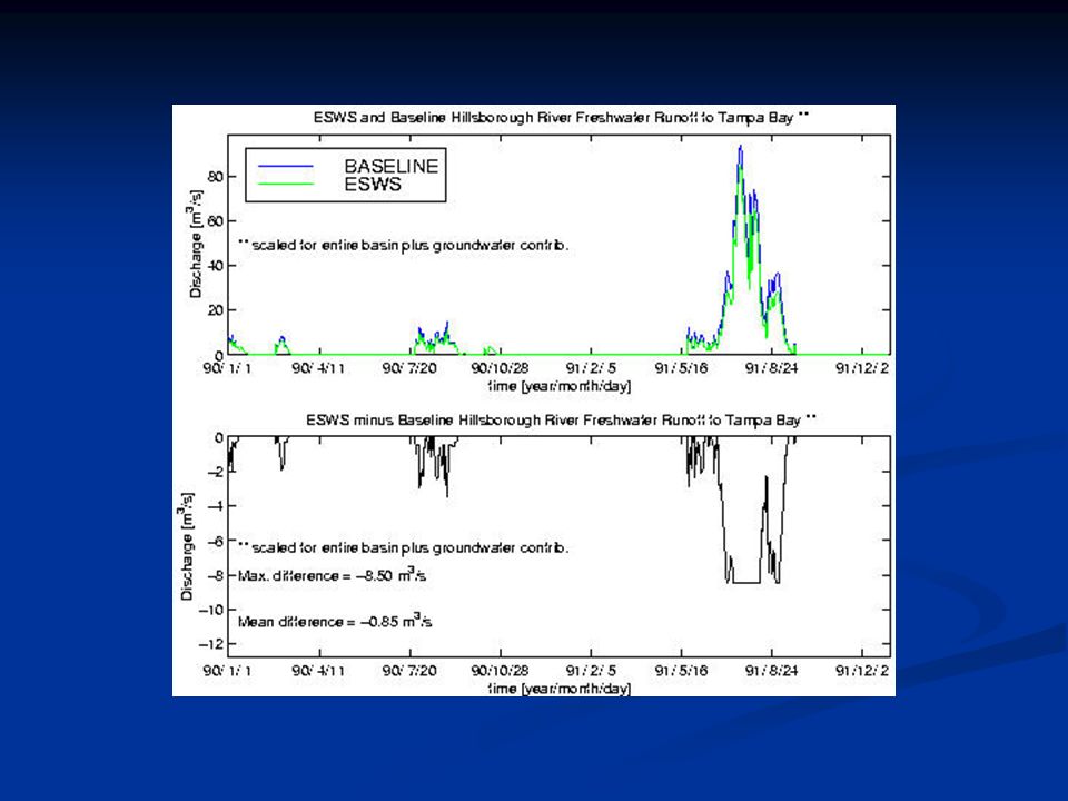
3. For Tampa Bay: Bay Volume = 3.8147 x 10 9 m 3 = 1.008 x 10 12 gal. = 1008 billion gal. Bay Area = 1,031 km 2 = 1.031 x 10 9 m 2 Ave. Bay Depth = 3.7 m = 12.4 ft Deepest part of the bay is approx. 20 m = 67 ft Bay Length = 53 km Shoreline length: over 1,450 km Tidal Range = 0.7 m = 2.34 ft (difference between high and low tide) Tidal Prism = Tidal Range x Bay Area = 7.217 x 10 8 m 3 = 191 billion gal = 19% of Bay Volume (amount of water flowing in/out of the bay on one tidal cycle) Volume of fresh water entering bay: approx. 60 m 3 s -1 = 1369.4 MGD

4. Fraction Fresh water method: Fraction Fresh water method: V: Volume of Estuary R: River inflow S o : Salinity at the mouth S e : Average salinity of estuary V fw : volume of fresh water in estuary Time for all the fresh water in an estuary to be replaced by river inflow – Assumes that river inflow mixed evenly throughout estuary. In reality, much more complicated – Tampa Bay model For Tampa Bay: tidal prism method gives 3-7 days fraction fresh water method gives 40-120 days Other definitions: Bay Volume/Residual Circulation ~ 45 days Bay length/mean tidal excursion ~ 7 days Residence Time varies with where you are in the bay and when you look

5. Estuarine Circulation Pressure gradient force = friction force Pressure gradient force = friction force

6. Separate pressure gradient into external (barotropic) and internal (baroclinic): Separate pressure gradient into external (barotropic) and internal (baroclinic):

7. Pressure as a function of depth (z) at two locations along the axis of the bay. Pressure difference drives residual flow and is due both to variation in elevation of the sea surface (external) and to variation in density of the water (internal). Tidal mixing stirs fresher water from the head of the bay with saltier water from the mouth, keeping density more or less constant with depth but increasing from head to mouth.

8. Total flow is driven by the sum of the external and internal pressure gradient forces and is into the bay at depth and out of the bay near the surface

9. In rectangular estuary, get 2 layer flow: In rectangular estuary, get 2 layer flow: 0 looking up “classic” picture out in head mouth mixing Strength of mean circulation depends on A z (or J) which is parameterization of all time- Dependent processes, i.e. tidal mixing

10. In V-shaped estuary, get lateral gradients: In V-shaped estuary, get lateral gradients: 00 0 in out In deeper part of estuary, baroclinic (internal) pressure gradient is stronger – dominates balance because z is larger In shallow flanks, barotropic pressure gradient dominates balance

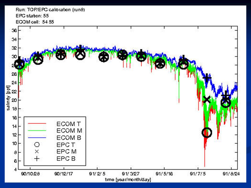
11. + Modeled (black) and Observed (red) current components (northward and eastward) averaged for December 1997 from the Port Manatee ADCP site. Red/black dotted lines are +/- ¼ standard deviation of the ADCP data Tampa Bay observed Residual Circulation from ADCP moorings

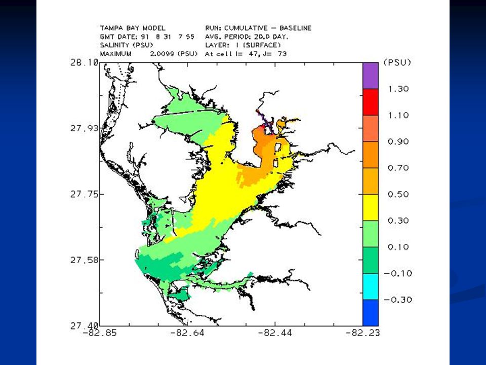
12. Average Bottom Salinity for August 31, 1991 Average salinity shows tongue of saltier water moving up ship channel …

13. Average Surface Salinity for August 31, 1991 … with fresher water moving out near the surface

14. Internal pressure gradient force drives flow into the bay in the deeper channels

15. External pressure gradient force drives flow out of the bay at shallower depths

16. Residence time is determined by the residual circulation and tidal mixing, and is shortest in the channels where circulation and mixing are strongest

17. Knudsen Relations V i : Residual circulation inflow w/ salinity S i V i : Residual circulation inflow w/ salinity S i V o : Residual circulation outflow w/ salinity S o V o : Residual circulation outflow w/ salinity S o V i S i =V o S o V i S i =V o S o V o - V i = X = R+P-E (net fresh water input) V o - V i = X = R+P-E (net fresh water input) V i =(X S o )/(S i - S o ) V i =(X S o )/(S i - S o ) V o =(X S i )/(S i - S o ) V o =(X S i )/(S i - S o ) If you know X, S i, S o, can estimate V i, V o If you know X, S i, S o, can estimate V i, V o

18. X=50 m 3 s -1 S o = 34 S i = 35 V i =(X S o )/(S i - S o ) = 1700 m 3 s -1 V o =(X S i )/(S i - S o ) = 1750 m 3 s -1 X

19. Residual Circulation Residence Time RT=strength of residual circulation across a section vs. volume bounded by that section RT=strength of residual circulation across a section vs. volume bounded by that section RT = Volume/V i RT = Volume/V i For Tampa Bay, Volume = 3.8147 x 10 9 m3 For Tampa Bay, Volume = 3.8147 x 10 9 m3 RT= 2.244 x 10 6 sec = 26 days RT= 2.244 x 10 6 sec = 26 days Compare with Volume-weighted average from Burwell (2000) Compare with Volume-weighted average from Burwell (2000)

20. In larger estuaries, Coriolis is not negligible – flow is concentrated to the right – in 2-layer flow: In larger estuaries, Coriolis is not negligible – flow is concentrated to the right – in 2-layer flow: Secondary transverse circulation

21. General Land Use Urban Ag & rural Wetlands & water Mining

22. Gaged and Ungaged Basins of the Tampa Bay Watershed

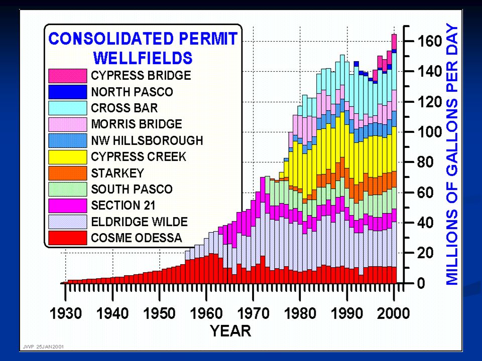
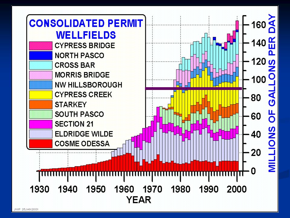
26. Permitted Surface Water Use

29. Real-time observations are combined with a model of currents and water level to provide a predictive capability for storm surge prediction and mitigation, search and rescue, environmental management/permitting, and hazardous material spills Sewage Spill Trajectory Desal Plant + + Piney Point Phosphate Plant Phosphate Discharge Trajectory

32. Big Bend Discharge

33. EPC Station 2