Download presentation
Presentation is loading. Please wait.

1
By Prof. Dr. Wail Nourildean Al-Rifaie

2
Basic principle of the moment distribution method
The frame shown in Fig. 1(a) is indeterminate to the sixth degree. If the rotation at joint ‘a’ is known, the internal forces could be determined. Hence, if it is assumed that the members are separated from each other as shown in Fig. 1(b) and that at the ends meeting at the joint ‘a’ the members have same rotation as the joint ‘a’ rotation Ɵ ( the compatibility condition at joint ‘a’ must be satisfied, i.e., Ɵab = Ɵac = Ɵd = Ɵ.
 is indeterminate to the sixth degree. If the rotation at joint ‘a’ is known, the internal forces could be determined. Hence, if it is assumed that the members are separated from each other as shown in Fig. 1(b) and that at the ends meeting at the joint ‘a’ the members have same rotation as the joint ‘a’ rotation Ɵ ( the compatibility condition at joint ‘a’ must be satisfied, i.e., Ɵab = Ɵac = Ɵd = Ɵ.")
4
Sign convention for fixed–end moments at the restrained ends
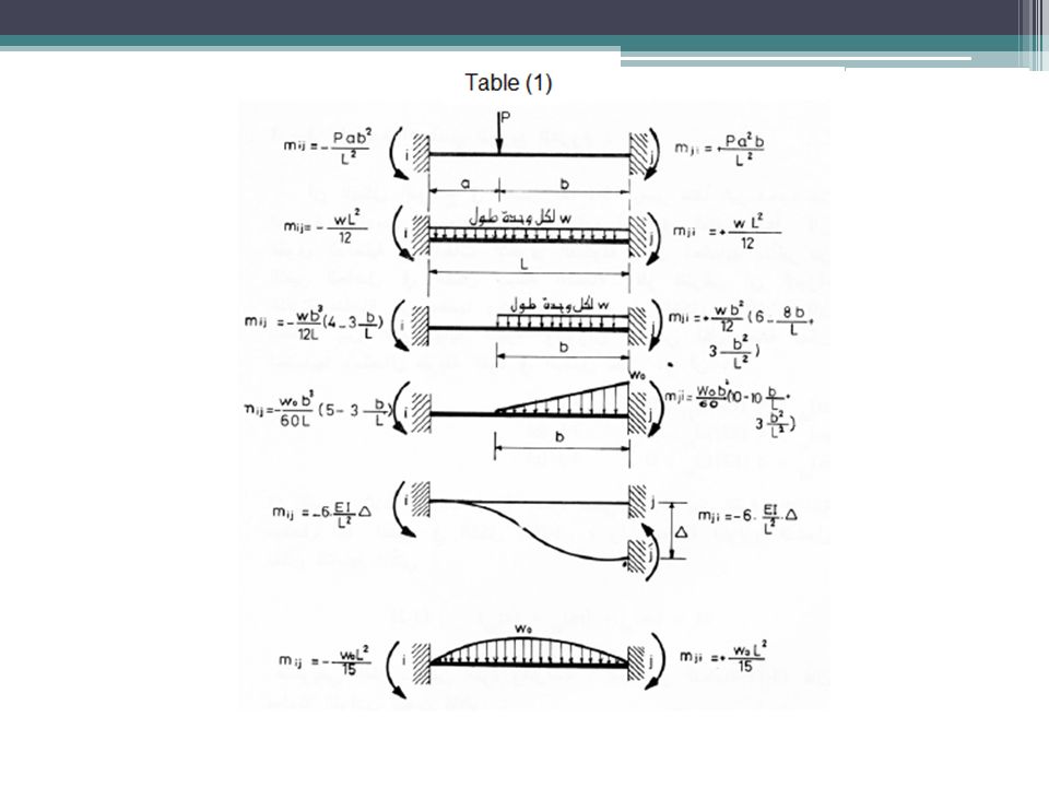
The moments induced at the two restrained ends of a loaded member are known as “Fixed-end moments” or F.E.M. The restrained ends do not permit rotation, i.e., Ɵ = 0. These fixed end moments can be determined using force method. Table 1 gives values of fixed-end moments for a number of common loading cases. A fixed-end moment is considered positive if it is clockwise and negative , if it is anticlockwise.

6
The relation between the end moment of the member and the corresponding rotation could be determined by using the force method of analysis which as follows:

7
The above three equations represent the force displacement relations at the joint ‘a’ as shown in the figure. By applying the equilibrium condition at joint ‘a’:

8
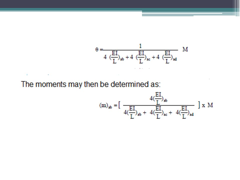
The rotation Ɵ may the determined as:

11
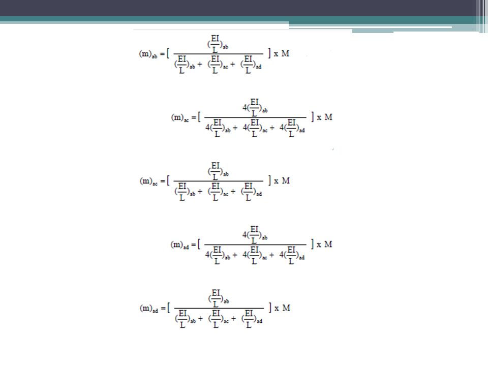
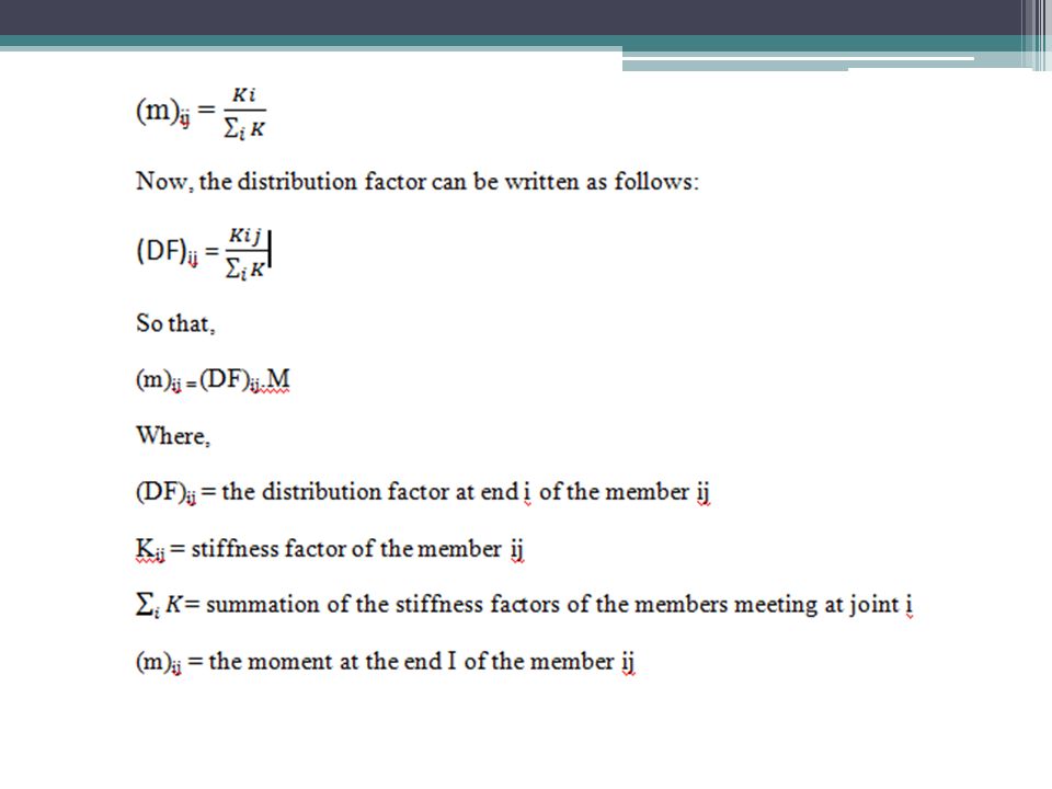
The quantity within the brackets [ ] in each of the above equations is called the “distribution factor” for the respective member and the value of 4EI/L represents the “stiffness factor” of the member. Putting K=4EI/L, the above equations can be represented as follows:
![The quantity within the brackets [ ] in each of the above equations is called the distribution factor for the respective member and the value of 4EI/L represents the stiffness factor of the member.](http://slideplayer.com/slide/9007045/27/images/11/The+quantity+within+the+brackets+%5B+%5D+in+each+of+the+above+equations+is+called+the+distribution+factor+for+the+respective+member+and+the+value+of+4EI%2FL+represents+the+stiffness+factor+of+the+member..jpg "Putting K=4EI/L, the above equations can be represented as follows: .")
13
Carry–over factor The propped cantilever beam shown in Fig. (2) is subjected to a moment Mab applied at joint ‘a’ in the clockwise direction. Moment Mab produces a rotation Ɵ at end (a) and a moment Mb is induced at the fixed end (b). By using force method the end moment Mb is: The direction of the moment Mb is clockwise, i.e. it has the same direction as the applied moment Mab. The coefficient, ½ is called the “carry-over factor”. The direction of the moment induced at the fixed end is the same as that of the applied moment. The carry-over factor depends on the “EI” value of the member. It may be noted that the value of +1/2 is true only for a prismatic member.
 is subjected to a moment Mab applied at joint ‘a’ in the clockwise direction. Moment Mab produces a rotation Ɵ at end (a) and a moment Mb is induced at the fixed end (b). By using force method the end moment Mb is: The direction of the moment Mb is clockwise, i.e. it has the same direction as the applied moment Mab. The coefficient, ½ is called the carry-over factor . The direction of the moment induced at the fixed end is the same as that of the applied moment. The carry-over factor depends on the EI value of the member. It may be noted that the value of +1/2 is true only for a prismatic member.")
14
Example 1: It is required to find moments at ‘a’ and ‘c’ of the frame shown in Fig. 2. the modulus of elasticity (E) is constant for the members of the frame.
 is constant for the members of the frame..")
15
Solution:

17
Technique of locking and unlocking:
The basis of moment distribution method consists in locking the joints in the structure and then unlocking them, allowing the joints to rotate (a moment is first applied externally to a joint in a beam/ frame for locking the joint, i.e., fixing the joint, and preventing it from rotation, and then concelling that moment by applying an equal and opposite moment and allowing the joint to rotate. Thus there is no residual moment on the actual structure because the two actionshave been neutralized.

18
The structure shown in Fig
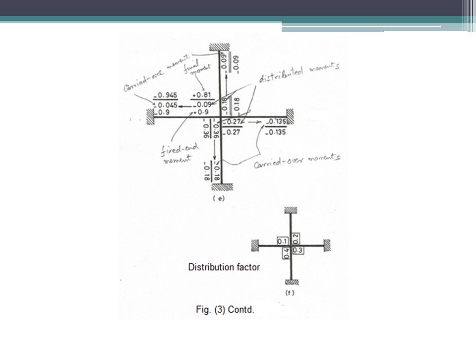
The structure shown in Fig. (3) has all its joints fixed except the joint ”e” which is free to rotate. Assume that a imaginary moment M is applied at joint “e” for locking and preventing it from rotation –see Fig. 4(b), i.e., Ɵ = 0, under the effect of the uniformly distributed load on the length ‘ae’. Due to this locking and resulting fixity of joint ‘e’, the members of the structure behave as separate ended beams and the two fixed end moments at each end of various members could be obtained from Table (1). The values of the fixed end moments on “ae” are: (F.E.M)ea = - (F.E.M)ae =(1.2)(3)^2/12 = 0.9kN.m
 has all its joints fixed except the joint e which is free to rotate. Assume that a imaginary moment M is applied at joint e for locking and preventing it from rotation –see Fig. 4(b), i.e., Ɵ = 0, under the effect of the uniformly distributed load on the length ‘ae’. Due to this locking and resulting fixity of joint ‘e’, the members of the structure behave as separate ended beams and the two fixed end moments at each end of various members could be obtained from Table (1). The values of the fixed end moments on ae are: (F.E.M)ea = - (F.E.M)ae =(1.2)(3)^2/12 = 0.9kN.m.")
21
In the other members of the structure, there are no fixed end moments as they do not have any transverse loads acting on them. By adding the fixed end moments at the member ends at joint ‘e’, the locking moment at joint ‘e’ is: And acts on the joint ‘e’ in the clockwise direction. This moment is called the ‘unbalanced moment’

22
2. Joint ‘e’ will now be released from the imaginary restraint by applying a moment equal in magnitude to the locking moment (M), but in the opposite direction. This can be called the unlocking moment, i.e., This unlocking moment will get distributed to the ends of the intersecting members at joint ‘e’ in the ratio of their distribution factors.
, but in the opposite direction. This can be called the unlocking moment, i.e., This unlocking moment will get distributed to the ends of the intersecting members at joint ‘e’ in the ratio of their distribution factors.")
24
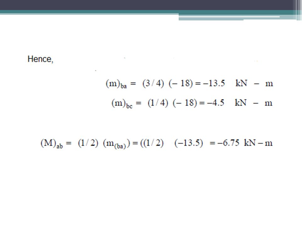
3. The far ends of the members intersecting at joint ‘e’ will be subjected to a moment equal to the distributed moment multiplied by the carry-over factor for that member. Since each member is uniform in cross-section, the carry-over factor is equal ½ for all members, and therefore,

25
4. By applying the equilibrium condition of moment at each joint, i. e
4. By applying the equilibrium condition of moment at each joint, i.e., the summation of moments at a joint =0. if this is not so, it means there is a residual locking moment at that joint. The next step consists in releasing the joint again and repeating the same procedure as in steps 2 and 3, until residuals are relatively small. 5. The final value of the moment at a joint will be obtained by taking the summation of the distributed and carried over moments as obtained in the above steps. See Fig. 3(e).
.")
26
Application to continuous beams
The basic steps for calculating the bending moments in continuous beams can be summarized as follows: The distribution factors, at each joint, for the ends of the intersecting members, are computed. As mentioned before, each member of the structure is assumed to be a fixed ended beam and the fixed end moments due to applied loads on the member re computed, using the sign convention referred to previously. The joints are released one at a time and the unbalanced moment is distributed at the intersecting end of each of the members meeting at the joint by the distribution factor for that member.

27
4. A member is induced at the far end of each member, which is equal to the distributed moment multiplied by the carry-over factor of that member. 5. Steps (3) and (4) are to be repeated for each joint until the relaxation effect of the joint is small and the unbalanced moment at the joint is negligible.
 and (4) are to be repeated for each joint until the relaxation effect of the joint is small and the unbalanced moment at the joint is negligible.")
28
Example: The continuous beam “abcd” shown in the figure, calculate the support moments and draw the shearing force and bending moment diagrams. The flexural rigidity ‘EI’ is constant for all the members.

30
Example: Determine the moments at the supports for beam shown in the figure, given that the modulus of elasticity is constant along the beam and the moment of inertia of each member is as shown in the figure.

32
Example: Analyze the beam “abcd” given in previous example using the modified stiffness factor for member “cd”.

33
The solution is shown below.

34
Moment distribution with known joint translation
Moment distribution as explained above is applicable in case there is no translation of any of the joints. However, due to the effect of the applied loads, the supports might yield or give way and displace by unequal amounts. The effect of this relative settlement between the supports can be accounted for in the moment distribution method by adding to the fixed end moments due to the applied loads, the fixed end moments due to the relative settlements of the supports. The moments may then be distributed in the same way as previously explained .

35
Example: The continuous shown in the figure has constant flexural rigidity ‘EI’ and is subjected to a uniformly distributed load on member ‘ab’. Also, there is a vertical settlement of support “c” equal to 30mm. Find moments in the beam.

37
Moment distribution for the analysis of structures with joint translations (sidesway)
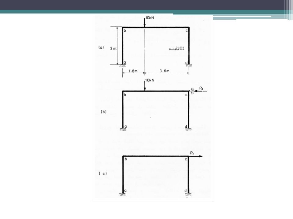
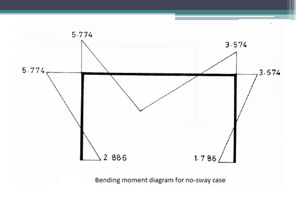
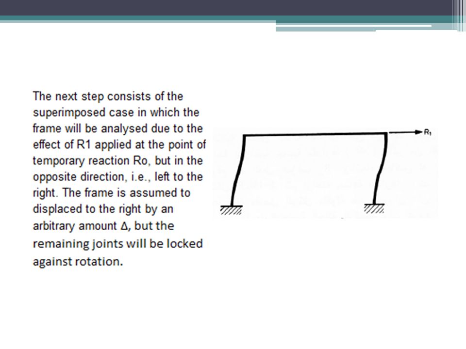
So far the effect of known joint translations (relative settlements) has been considered due to which moments are induced at the restrained ends. The usual steps are then carried out by the moment distribution method and the final moments at the joints are obtained. But there are structures which are free to translate by unknown amounts. For the frame shown in the following Fig. (A), member ‘b’ has freedom of sidesway translation with bending in the members. This frame can be replaced by two other separate frames shown in Figs. (B) and (C) respectively. The principle of superposition is applied to obtained the final solution. In the frame show in Fig.(b), the two joints (c) and (b) are prevented against sidesway by support at (c), and the analysis will proceed in the usual manner. Due to the temporary restraint, there will be a reaction in the direction of the restraint at joint(c) equal to Ro. The reaction Ro at c does not produce any fixed-end moments in any member. This can be called the non sway case and is shown in Fig. (b). The second case is obtained by removing the temporary restraint and applying a lateral force at the location of the temporary restraint equal and opposite to the reaction at the restraint, as shown in Fig. (c). This case be called the superimposed case, R1 causes unknown sidesway and hence the fixed end moments can not be calculated directly. It is
 has been considered due to which moments are induced at the restrained ends. The usual steps are then carried out by the moment distribution method and the final moments at the joints are obtained. But there are structures which are free to translate by unknown amounts. For the frame shown in the following Fig. (A), member ‘b’ has freedom of sidesway translation with bending in the members. This frame can be replaced by two other separate frames shown in Figs. (B) and (C) respectively. The principle of superposition is applied to obtained the final solution. In the frame show in Fig.(b), the two joints (c) and (b) are prevented against sidesway by support at (c), and the analysis will proceed in the usual manner. Due to the temporary restraint, there will be a reaction in the direction of the restraint at joint(c) equal to Ro. The reaction Ro at c does not produce any fixed-end moments in any member. This can be called the non sway case and is shown in Fig. (b). The second case is obtained by removing the temporary restraint and applying a lateral force at the location of the temporary restraint equal and opposite to the reaction at the restraint, as shown in Fig. (c). This case be called the superimposed case, R1 causes unknown sidesway and hence the fixed end moments can not be calculated directly. It is.")
39
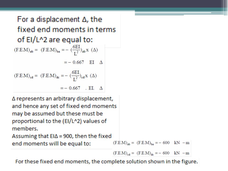
Therefore necessary to assume an arbitrary known displacement ∆ in the direction of the unknown force R1 which causes the displacement. It is then possible to calculate the unknown force R1 required to cause the displacement and the resulting moments. The superposition principle is then applied by adding the moments due to the non-sway case to those due to the superimposed case so that the equilibrium condition ∑Fx=0 is satisfied at the location of the imaginary restraint. There is thus now no restraint after the addition of the superimposed case on the non-sway case. See figs. (b) and (c).
 and (c)..")
40
Example: It is required to draw the bending moment diagram for the frame shown.

41
Solution Step 1:

44
The next step is to determine the temporary restraint reaction Ro as follows:

48
The following figures show the method of determination of values of R1.

Similar presentations


>")


 Chapter 4: Deformation of Statically Determinate Structure (Beam Deflection) Shahrul Niza Mokhatar shahruln@uthm.edu.my.>")


