1. Copyright © 2006 The McGraw-Hill Companies, Inc. All rights reserved. McGraw-Hill/Irwin Review of Statistics I: Probability and Probability Distributions chapter two

2. 2-2 Notation and Definitions Summation Sign Σ The sum of the variable X from the first value, i = 1, to the last value, i = n, where n is the last value.

3. 2-3 Definitions Statistical or Random Experiment Any process of observation or measurement That has more than one possible outcome For which there is uncertainty about the outcome Examples: tossing a coin, drawing cards from a deck. Sample Space or Population The set of all possible outcomes of an experiment What is the sample space for tossing two fair coins? Sample Point Each individual outcome or member of the sample space

4. 2-4 Definitions Event A particular collection of outcomes A subset of the sample space Events are Mutually exclusive if the occurrence of one prevents the occurrence of another Equally likely if one is just as likely to occur as another Collectively exhaustive if they exhaust all possible outcomes of an experiment.

5. 2-5 Example Suppose the MTSU baseball team is playing a doubleheader. It terms of winning or losing each game, there are four possible outcomes for MTSU: WW, WL, LW, LL. Note that each outcome is an event. What is the sample space? Are the events: mutually exclusive? equally likely? collectively exhaustive?

6. 2-6 Figure 2-1 Venn diagram.

7. 2-7 Venn Diagram The rectangle is the sample space The circles represent events Fig. 2-1(a): outcomes that belong to A and its complement A’ Fig. 2-1(b): Union of A and B, A U B Fig. 2-1(c): Intersection of A and B, A ∩ B Fig. 2-1(d): A and B are mutually exclusive How can you represent number of MTSU baseball wins?

8. 2-8 Random Variables A variable whose numerical value is determined by the outcome of an experiment. Example: Toss two coins and observe the number of heads. Possible outcomes are TT0 TH1The number of heads is a random HT1variable (as is MTSU’s number of wins). HH2 These are discrete random variables that are countable. Continuous r.v.’s can take any value within a range (such as the height or weight of students in this class).

9. 2-9 Classical Probability Classical or A Priori definition If an experiment can result in n mutually exclusive and equally likely outcomes And if m outcomes are favorable to event A Then the probability of A, P(A), is m/n P(A) = (number of outcomes favorable to A) (total number of outcomes) Examples: coin toss, dice roll, card draw.

10. 2-10 Empirical Probability Relative Frequency or Empirical Definition The number of occurrences of a given event divided by the total number of occurrences. Or, relative frequency = absolute frequency divided by total number of occurrences. If in n trials, m are favorable to A, then P(A) = m/n, if n is sufficiently large. “Large” depends on context. Example: frequency distribution of eye color among MTSU students.

11. 2-11 Properties of Probabilities 0 < P(A) < 1 If A, B, C,…are mutually exclusive events P(A + B + C+…) = P(A) + P(B) + P(C)…. The probability that any one of these events occurs is the sum of their individual probabilities. If A, B, C, …are mutually exclusive and a collectively exhaustive set of events P(A + B + C+…) = P(A) + P(B) + P(C)….= 1

12. 2-12 Some Rules of Probability The events A, B, C,…are said to be statistically independent if the probability that they occur together is the product of their individual probabilities. P(ABC…) = P(A)P(B)P(C)…. P(ABC…) is the probability of events ABC… occurring simultaneously or jointly, called a joint probability. P(A), P(B), P(C),…are called unconditional, marginal or individual probabilities. Example: Toss two coins. What is the probability of a head on the first coin and a head on the second coin?

13. 2-13 Some Rules of Probability If events A, B, C,…are not mutually exclusive P(A + B) = P(A) + P(B) – P(AB) Where P(AB) is the joint probability that A and B occur together. For every event A there is an event A’, the complement of A, where P(A + A’) = 1 P(AA’) = 0

14. 2-14 Conditional Probability The probability that event A occurs knowing that event B has occurred The conditional probability of A, conditional on event B occurring, is P(A|B) = P(AB)/P(B) for P(B) > 0; And P(B|A) = P(AB)/P(A) for P(A) > 0 Example: 300 males and 200 females take an accounting class. Of these, 100 males and 60 females are accounting majors. If a student chosen at random from the class is an accounting major, what is the probability that the student is male?

15. 2-15 Conditional Probability Conditional and unconditional probabilities are generally different, unless the two events are independent, then P(A|B) = P(AB)/P(B) = [P(A)P(B)]/P(B) = P(A) Since P(AB) = P(A)P(B) when the two events are independent.

16. 2-16 Bayes’ Theorem Use the knowledge that an event B has occurred to update the probability that an event A has occurred. P(A|B) = P(B|A)P(A) P(B|A)P(A) + P(B|A’)P(A’) Where A’ is the complement of A P(A) is called the prior probability P(A|B) is called the posterior probability

17. 2-17 Bayes’ Theorem Example: Suppose a woman has two coins in her purse, one is fair and one is two-headed. She takes a coin at random from her purse and tosses it. A head shows up. What is the probability that the coin is two headed?

18. 2-18 Random Variables Probability Random variables are numerical representations of the outcomes or events of a sample space Since we can assign probabilities to outcomes and events, we can assign probabilities to random variables. Probability Distributions The possible values taken by a random variable and the probabilities of occurrence of those values.

19. 2-19 Discrete Random Variables Probability Mass Function (PMF) For a discrete r.v. X taking values x 1, x 2,…. f(X = x i ) = P(X = x i )i = 1, 2, …. is the PMF or probability function (PF). Properties of PMF or PF 0 < f(x i ) < 1 ∑ x f(x i ) = 1

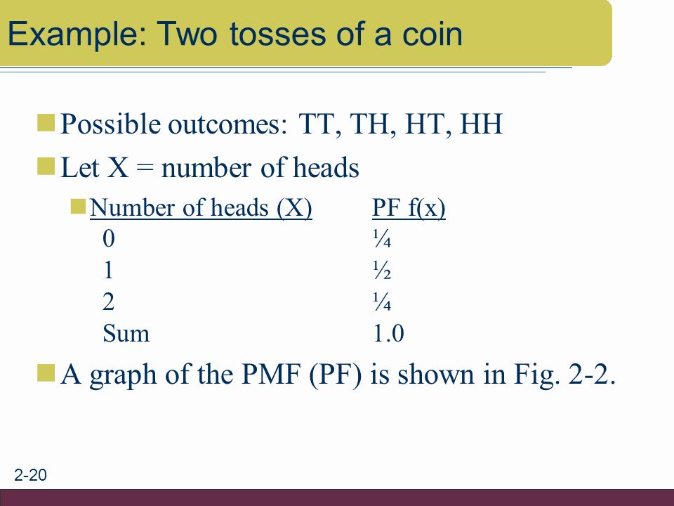
20. 2-20 Example: Two tosses of a coin Possible outcomes: TT, TH, HT, HH Let X = number of heads Number of heads (X)PF f(x) 0¼ 1½ 2¼ Sum1.0 A graph of the PMF (PF) is shown in Fig. 2-2.

21. 2-21 Figure 2-2 The probability mass function (PMF) of the number of heads in two tosses of a coin (Example 2.13).

22. 2-22 Continuous Random Variables Probability Density Function (PDF) A continuous r.v. can take an uncountably infinite number of values The probability that a continuous r.v. takes a particular value is always zero The probability for a continuous r.v. is always measured over an interval x2 P(x 1 < X < x 2 ) = ∫ x1 f(x)dx See Fig. 2-3

23. 2-23 Figure 2-3 The PDF of a continuous random variable.

24. 2-24 Continuous Random Variables Since P(X = x 1 ) = 0, thenthe following are equivalent P(x 1 < X < x 2 )

25. 2-25 Cumulative Distribution Function (CDF) F(X) = P(X < x) or the probability that X takes a value less than or equal to x F(-∞) = 0 and F(∞) = 1 F(x) is nondecreasing, for x 2 > x 1 then F(x 2 ) > F(x 1 ) P(X > k) = 1 – F(k) P(x 1 < X < x 2 ) = F(x 2 ) – F(x 1 )

26. 2-26 Example: Number of Heads in 4 Tosses XValue XPDFValue XCDF 00 < X < 11/16X < 01/16 11 < X < 24/16X < 15/16 22 < X < 36/16X < 211/16 33 < X < 44/16X < 315/16 44 < X1/16X < 41

27. 2-27 Figure 2-4 The cumulative distribution function (CDF) of a discrete random variable (Example 2.15).

28. 2-28 Figure 2-5 The CDF of a continuous random variable.

29. 2-29 Multivariate PDFs Previous examples involved one r.v. and are single variable or univariate PDFs Outcomes of some experiments may be described by more than one r.v. These involve multivariate PDFs The simplest of these is the bivariate, or two variable, PDF Table 2-2 is an example of a joint frequency distribution for two variables.

30. 2-30 Table 2-2: Absolute Frequencies The frequency distribution of two random variables: Number of PCs sold (X) and Number of Printers sold (Y).

31. 2-31 Table 2-3: Measures of Joint Probabilities The bivariate probability distribution of number of PCs sold (X) and number of printers sold (Y).

32. 2-32 Bivariate or Joint PMF f(X, Y) = P(X = x and Y = y) is the joint PMF f(X, Y) = 0 when X ≠ x and Y ≠ y The probability that X and Y take certain values simultaneously f(X, Y) > 0 for all pairs of X and Y ∑ x ∑ y f(X, Y) = 1 sum of joint probabilities Leads to Marginal and Conditional PFs

33. 2-33 Marginal Probability Distributions f(X) and f(Y) are called univariate, unconditional, individual, or marginal PMFs or PDFs relative to the joint or bivariate PF f(X, Y). For example, the marginal PMF of X is the probability that X takes a given value regardless of the values taken by Y Tables 2-3 and 2-4 show how the marginal PMF is derived

34. 2-34 Table 2-4 Marginal probability distributions of X (number of PCs sold) and Y (number of printers sold).

35. 2-35 Conditional Probability Functions What is the probability that Y = 4, conditional on X = 4 (Table 2-3)? This known as a conditional probability and be found from the conditional PMF f(Y | X) = P(Y = y | X = x) and f(X | Y) = P(X = x | Y = y) These can be computed as f(Y | X) = f(X, Y)/f(X) and f(X | Y) = f(Y, X)/f(Y) Or conditional = joint/marginal of conditioning r.v.

36. 2-36 Statistical Independence Two variables, X and Y, are statistically independent if and only if their joint PMF or PDF can be expressed as the product of their individual or marginal PMFs or PDFs for all combinations of X and Y. Example: A bag contains three balls numbered 1, 2, 3. Two balls are drawn at random with replacement. X is the number on the first ball and Y is the number on the second. Consider f(X = 1, Y = 1), f(X = 1), and f(Y = 1) from Table 2-5. Are the number of PCs and printers sold in Table 2-3 independent random variables?

37. 2-37 Table 2-5 Statistical independence of two random variables.