Download presentation
Presentation is loading. Please wait.

1
Additional Topics in Prediction Methodology

2
Introduction Predictive distribution for random variable Y 0 is meant to capture all the information about Y 0 that is contained in Y n. not completely specify Y 0 but does provide a probability distribution of more likely and less likely values of Y 0 E{Y 0 |Y n } is the best MSPE predictor of Y 0

3
Hierarchical models have two stages X R d f 0 =f(x 0 ) known p*1 vector F=(f j (x j )) known n*p matrix unknown p*1 vector regression coefficients R=(R(x i -x j )) known n*n matrix correlations among trainning data Y n r 0 =(R(x i -x 0 )) known n*1 vector correlations of Y 0 with Y n
 known p*1 vector F=(f j (x j )) known n*p matrix unknown p*1 vector regression coefficients R=(R(x i -x j )) known n*n matrix correlations among trainning data Y n r 0 =(R(x i -x 0 )) known n*1 vector correlations of Y 0 with Y n")
4
Predictive Distributions when Z 2, R and r 0 are known

6
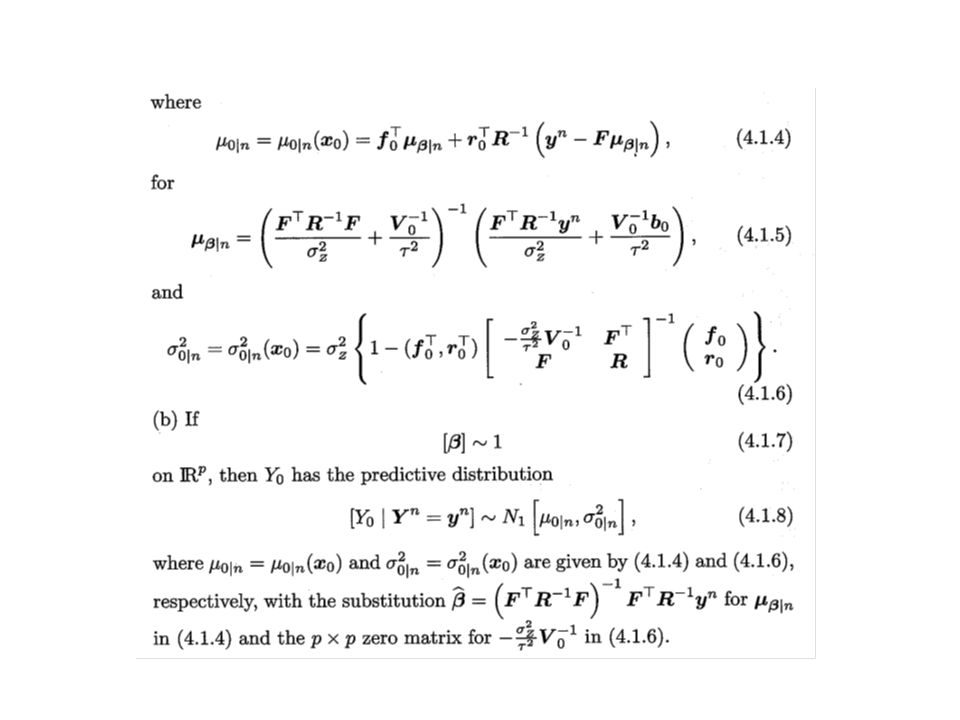
Interesting features of (a) and (b) Non-informative Prior is the limit of the normal prior as While the prior is non-informative, it is not a proper distribution. The corresponding predictive distribution is proper. The same conditioning argument can be applied to drive posterior mean for the non-informative prior and normal prior.

7
The mean and variance of the predictive distribution (mean) 0|n (x 0 ) and 0|n (x 0 ) depend on x 0 only through the regression function f 0 and correlation vector r 0 0|n (x 0 ) is a linear unbiased predictor of Y(x 0 ) The continuity and other smoothness properties of 0|n (x 0 ) are inherited from correlation function R(.) and the regressors {f(.)} j=1 p
 0|n (x 0 ) and 0|n (x 0 ) depend on x 0 only through the regression function f 0 and correlation vector r 0 0|n (x 0 ) is a linear unbiased predictor of Y(x 0 ) The continuity and other smoothness properties of 0|n (x 0 ) are inherited from correlation function R(.) and the regressors {f(.)} j=1 p")
8
0 |n(x 0 ) depends on the parameters z 2 2 only through their ratio 0 |n(x 0 ) interpolate the training data. When x 0 =x i, f 0 =f(x i ), and r 0 T R -1 =e i T, the i th unit vector.
, and r 0 T R -1 =e i T, the i th unit vector..")
10
The mean and variance of the predictive distribution (Variance) MSPE( 0 |n(x 0 ) )= 0|n 2 (x 0 ) The variance of the posterior of Y(x 0 ) given Y n should be 0 whenever x 0 =x i 0|n 2 (x i )=0
 MSPE( 0 |n(x 0 ) )= 0|n 2 (x 0 ) The variance of the posterior of Y(x 0 ) given Y n should be 0 whenever x 0 =x i 0|n 2 (x i )=0")
11
Most important use of Theorem 4.1.1

12
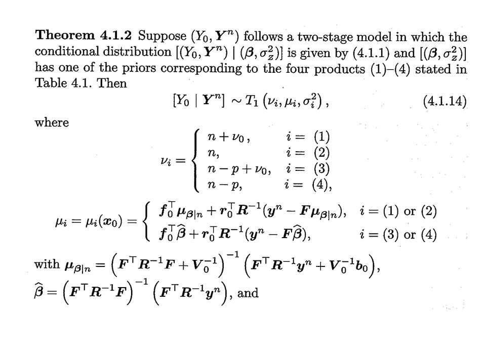
Predictive Distributions when R and r 0 are known The posterior is a location shifted and scaled univariate t distribution having degrees of freedom that are enhanced when there is informative prior information for either or z 2

15
Degree of freedom Base value for the degree of freedom i =n-p P additional degrees of freedom when prior is informative 0 additional degree of freedom when z 2 is informative

16
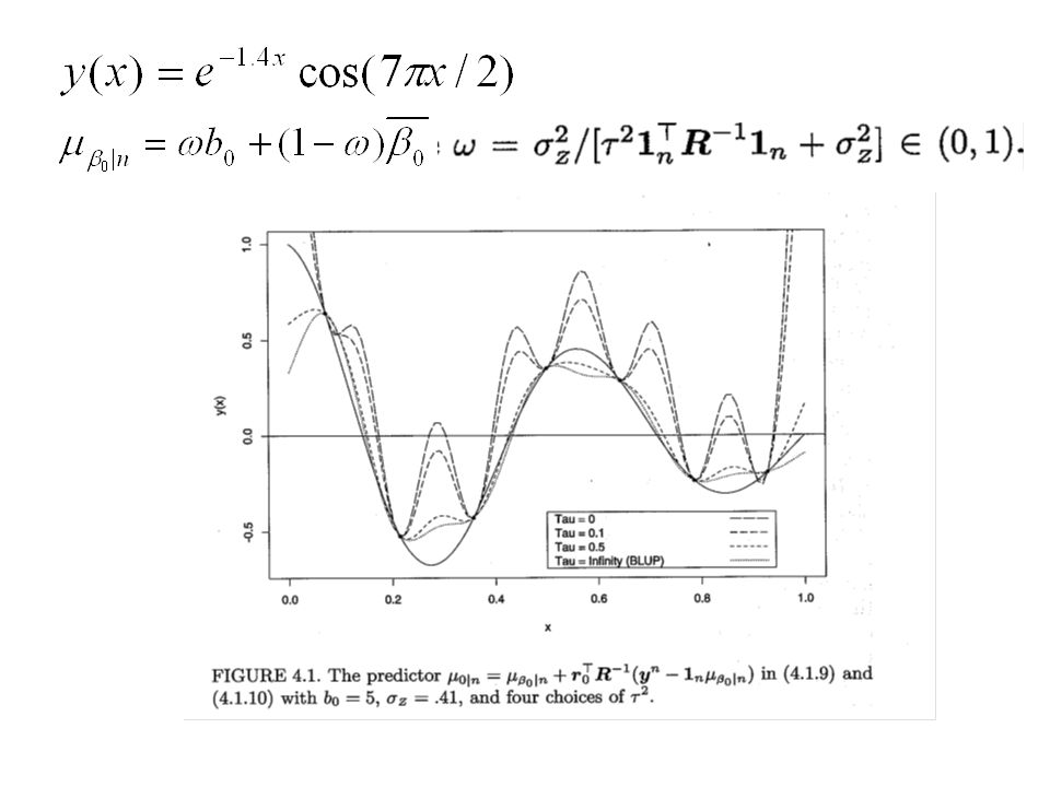
Location shift The same centering value as Theorem 4.1.1 (known z 2 ) The non-informative prior gives the BLUP
 The non-informative prior gives the BLUP")
17
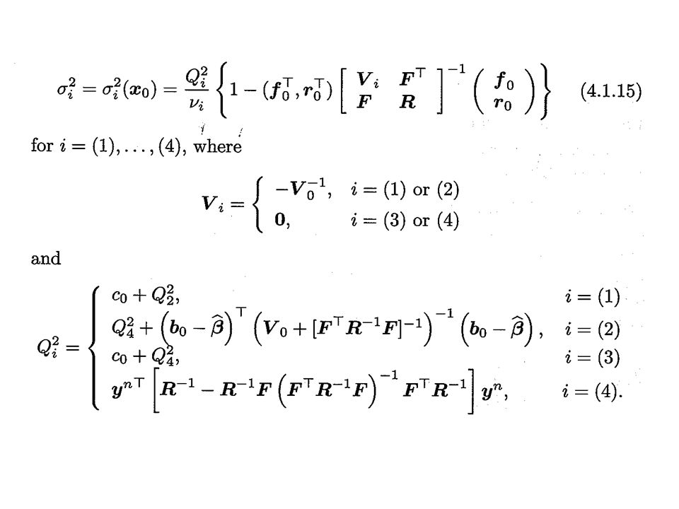
Scale factor i 2 (x 0 ) (compare 4.1.15 with 4.1.6) Estimate of the scale factor 0|n 2 (x 0 ). Q i 2 / i : estimate z 2 Q i 2 : get information about z 2 from the conditional distribution Y n given z 2 and information from the prior of z 2 i 2 (x i )=0, x i is any of the training data points.
=0, x i is any of the training data points..")
18
Prediction Distributions when Correlation parameters are unknown If the correlations among the observations is unknown (R r 0 are unknown)? –Assume y(.) has a Gaussian prior with correlation function R(.| ), is unknown vector parameters Two issues –Standard error of Plug-in predictor 0|n (x 0 | ) by substituting comes from MLE or REML –Bayesian approach to uncertainty in which is to model it by a prior distribution
 has a Gaussian prior with correlation function R(.| ), is unknown vector parameters Two issues –Standard error of Plug-in predictor 0|n (x 0 | ) by substituting comes from MLE or REML –Bayesian approach to uncertainty in which is to model it by a prior distribution.")
19
Prediction of Multiple Response Models Several outputs are available for from a computer experiment Several codes are available for computing the same response (fast and slow code) Competing response Several stochastic models for joint response Using these models to describe the optimal predictor for one of the several computed responses.
 Competing response Several stochastic models for joint response Using these models to describe the optimal predictor for one of the several computed responses.")
20
Modeling Multiple Outputs Z i (.): marginally mean zero stationary Gaussian stochastic processes with unknown variance and correlation function R Z i (x) implies that the correlation between Z i (x 1 ) and Z i (x 2 ) only depends on x 1 -x 2 Assume Cov(Z i (x 1 ), Z j (x 2 ))= i j R ij (x 1 -x 2 ) R ij (.) cross-correlation function of Z i (.) and Z j (.) Linear model: global mean of the Y i process. f i (.): known regression functions i : unknown regression parameters
: known regression functions i : unknown regression parameters.")
21
Selection of correlation and cross- correlation functions are complicated Reason: for any input sites xli, the multivariate normal distributed random vector (Z 1 (x 1 1 ), ….) T must have a nonnegative definite covariance matrix Solution: construct the Z i (.) from a set of elementary processes (usually this processes are mutually independent)
, ….) T must have a nonnegative definite covariance matrix Solution: construct the Z i (.) from a set of elementary processes (usually this processes are mutually independent)")
22
Example by Kennedy and O’Hagan Y i (x): prior for the i th code level (i=m top-level code). The autoregressive model: –Y i (x)= i-1 Y i-1 (x)+ i (x), i=2, …, m The output for each successive higher level code i at x is related to the output of the less precise code i-1 at x plus the refinement i (x) –Cov(Y i (x), Y i-1 (w)|Y i-1 (x))=0 for all w~=x No additional second-order knowledge of code i at x can be obtained from the lower-level code i-1 if the value of code i-1 at x is known (Markov property on the hierarchy of codes) Since there is no natural hierarchy of computer code in such applications, we need find something better.
= i-1 Y i-1 (x)+ i (x), i=2, …, m The output for each successive higher level code i at x is related to the output of the less precise code i-1 at x plus the refinement i (x) –Cov(Y i (x), Y i-1 (w)|Y i-1 (x))=0 for all w~=x No additional second-order knowledge of code i at x can be obtained from the lower-level code i-1 if the value of code i-1 at x is known (Markov property on the hierarchy of codes) Since there is no natural hierarchy of computer code in such applications, we need find something better..")
23
More reasonable Model Each constraint function is associated with the objective function plus a refinement –Y i (x)= i Y 1 (x)+ i (x), i=2, …, m+1 Ver Hoef and Marry –Form models in the environmental sciences –Include an unknown smooth surface plus a random measurement error. –Moving averages over white noise processes

24
Morris and Mitchell model Prior information about y(x) is specified by a Gaussian processor Y(.) Prior information about the partial derivatives y (j) (x) is obtained by considering the “derivative” processes of Y(.) –Y1(.)=y(.), y2(.)= y (1) (.), y 1+m (.)=y (m) (.) Natural prior for y(j)(x): The covariances between Y(x 1 ), Y (j) (x 2 ) and Y (i) (x 1 ), Y (j) (x 2 ) are:
 is specified by a Gaussian processor Y(.) Prior information about the partial derivatives y (j) (x) is obtained by considering the derivative processes of Y(.) –Y1(.)=y(.), y2(.)= y (1) (.), y 1+m (.)=y (m) (.) Natural prior for y(j)(x): The covariances between Y(x 1 ), Y (j) (x 2 ) and Y (i) (x 1 ), Y (j) (x 2 ) are:")
25
Optimal Predictors for Multiple Outputs The best MSPE predictor based on training data is: Where Y 0 =Y 1 (X 0 ), Y i ni =(Y i (x 1 i ), …), and y i ni is observed value for i=[1,m]
![Optimal Predictors for Multiple Outputs The best MSPE predictor based on training data is: Where Y 0 =Y 1 (X 0 ), Y i ni =(Y i (x 1 i ), …), and y i ni is observed value for i=[1,m]](http://images.slideplayer.com/27/8931395/slides/slide_25.jpg "Optimal Predictors for Multiple Outputs The best MSPE predictor based on training data is: Where Y 0 =Y 1 (X 0 ), Y i ni =(Y i (x 1 i ), …), and y i ni is observed value for i=[1,m]")
26
The joint distribution is the multivariate normal distribution

27
Conditional expectation ….. In practice, this is useless (it requires knowledge of marginal correlation functions, joint correlation function and ratio of all the process variance) Empirical versions are of practical use: –Every time we assume each of the correlation matrices R i and cross-correlation matrices R ij are known up to a vector of parameters. –Estimate using MLE or REML
 Empirical versions are of practical use: –Every time we assume each of the correlation matrices R i and cross-correlation matrices R ij are known up to a vector of parameters. –Estimate using MLE or REML.")
28
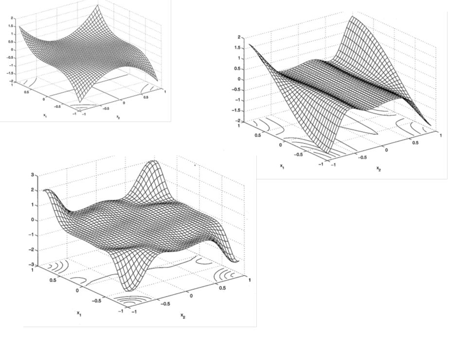
example1 14 point training data has feature that it allows us to learn over the entire input space: space-filling Compare two model –Using the predictor of y(.) based on y(.) alone –Using the predictor of y(.) base on (y(.), y (1) (.), y (2) (.)) Second one is both more visually fit and has 24% smaller ERMSPE
 based on y(.) alone –Using the predictor of y(.) base on (y(.), y (1) (.), y (2) (.)) Second one is both more visually fit and has 24% smaller ERMSPE")
30
Thank you!

Similar presentations