1. Economic Growth IN THE UNITED STATES OF AMERICA A County-level Analysis

2. What was our objective? To explore the factors driving differences in regional economic growth across the United States To apply the analysis in “The Sources of Economic Growth in OECD Regions: A Parametric Analysis” (December 2008) on United States counties

3. Agenda 1.Theory 2.Data 3.Summary Statistics 4.Results 5.Findings 6.Recommendations 7.Questions

4. Theory

5. What theories explain economic growth? 1. Neo-Classical Theory 2. Endogenous Growth Theory 3. New Economic Geography (NEG)

6. Neo-Classical Theory assumes exogenous technology Key assumptions Capital is subject to diminishing returns Perfect competition An exogenously determined constant rate reflects the progress made in technology Key factors Capital intensities Human capital Technology

7. Neo-Classical Theory predicts convergence Long-run growth is the result of continuous technological progress Key implication: Conditional convergence Problems Limited empirical evidence of convergence No room to capture fluctuations in technology and innovation

8. Endogenous Growth Theory assumes diminishing returns and endogenous technology Key assumptions Capital is subject to diminishing returns Sometimes imperfect competition Key factors Physical capital Human capital Technology (included in the model: endogenous)

9. Endogenous Growth Theory predicts that investment in human capital and R&D produce growth Key implication: policies that embrace openness, competition, change, and innovation will promote growth Theory emphasizes that private investment in R&D is the central source of technological progress No convergence is predicted Investment in human capital New technology, more efficient production Economic growth

10. New Economic Geography: Why is manufacturing concentrated in a few regions? Economic geography: the location of factors of production in space Key implication: despite early similarity, regions can become quite different Key factors causing agglomeration or dispersion Economies of scale Transportation costs Location of demand Population

11. New Economic Geography predicts that the right mix of factors causes growth and differentiation between regions One region is slightly larger Lower transportation costs Increasing returns to scale Larger initial production More people More production closer together

12. How does NEG differ from Neo-Classical and Endogenous Growth Theories? Takes scale into account External increasing returns to scale incentivizes agglomeration Agglomeration captures, via scale effects, how small initial differences cause large growth differentials over time

13. Data

14. We obtained data on 3,079 counties from 1998 to 2007 VariableSourceYear(s) Annualized Per Capita Personal Income Growth Bureau of Economic Analysis1998-2007 Log of Initial IncomeBureau of Economic Analysis1998 InfrastructureESRI Data and Maps 9.3 Media Kit2008 Education RatesU.S. Census2000 Innovation IndexEconomic Development Administration2008 Employment RateU.S. Census2000 Employment SpecializationCensus of Employment and Wages1998 Distance to MarketsESRI Data and Maps 9.3 Media Kit Bureau of Economic Analysis 2008 1998

15. The Equation Economic Growth = β 0 + β 1 Log of Initial Income + β 2 Infrastructure + β 3 Education Rates + β 4 Innovation Index + β 5 Employment Rate + β 6 Employment Specialization + β 7 Distance to Markets + ε

16. Summary Statistics

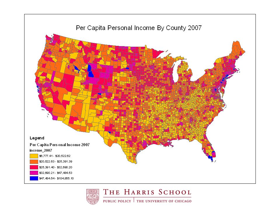
17. Per Capita Personal Income VariableHighestLowestMedian Annualized Per Capita Personal Income Growth 7.03% in Sublette, WY -3.55% in Crowley, CO 1.03% Income in Initial Year (1998) $76,450 in New York, NY $7,756 in Loup, NE $20,647

21. Infrastructure A measure of Physical Capital. Mileage of major roads by county to its population OECD used motorways density (total motorway kilometers in a region to its population)

22. Major Road Mileage by County

23. Education Rates VariableHighestLowestMedian Less than High School Diploma 62.5% in Starr, TX 4.4% in Douglas, CO 21.6% High School Diploma 53.5% in Carroll, OH 12.4% in Arlington, VA 34.7% More than High School Diploma 82.1% in Los Alamos, NM 17.2% in McDowell, WV 41.4% Total97.7%

24. Percent of population with more than a high school diploma

25. Innovation Index [COMING SOON]

26. Employment Rate VariableHighestLowestMedian Youth Employment Rate (16 – 20 years old ) 100% in Loving, TX 8.8% in Shannon, SD 46.2% Working-Age Employment Rate (21 – 65 years old) 88.4% in Stanley, SD 35.9% in McDowell, WV 73.1% Total Employment Rate 86.7% in Stanley, SD 33.6% in McDowell, WV 69.9%

27. Total employment rate

28. Employment Specialization What is it? Measure of industrial concentration of a region (county) What is it meant to capture? Captures notion of agglomeration What is agglomeration? The close spatial concentration of industry A determinant of economic growth in NEG growth theory How is it modeled? Specialization indices Herfindahl Index Krugman Index

29. Employment Specialization: Herfindahl Index Definition: N Σ i=1 s 2 Features: Ranges from 0 to 1.0 0 = industrial diversity (lots of firms) 1 = lack of industrial diversity (one or few firms) Is an absolute measure; Does not take neighbors into account

30. Employment Specialization

31. Employment Specialization: Krugman Index Definition: KI = ∑ j |a ij -b -ij | a = the share of industry j in county i’s total employment b = the share of the same industry in the employment of all other counties, -i KI = the absolute values of the difference between these shares, summed over all industries Features: Ranges from 0 to 2.0 0 = county i has industrial composition identical to its comparison counties 2 = county i has industrial composition without any similarity (no common industries) to its comparison counties Is a relative measure; Compares to one’s neighbors. It’s our choice!

32. Employment Specialization

35. Distance to Markets [INSERT]

36. Results

37. OLS Results Dependent variable: Annualized Per Capita Personal Income Growth 123456 Constant.0447189.0584573.1205336.0267810.02596360.076408 (.008105)(.0084161)(.0096707)(.0092717)(0.0094317)(0.011069) Initial Income-.003360.0026-.0109003-.0007123-0.0016588-0.0068127 (.0008151)(10.84)(.0010488)(.0010536)(0.0009249)(0.0011989) Highways2.67e-074.21e-07 (7.79e-07)(7.73e-07) Airports.0020899.0011322 (.0004307)(.000428) High school diploma-.0231712-.0102969 (.0035923)(.0042081) More than high school.0169572.0222506 (.0025776)(.0030055) Employment Rate-.0121145 (.0030641) Krugman Index0.0022827.0032505 (0.0005908)(.0006539) Distance to Markets R-Squared0.08970.01730.07460.01050.01030.0997 F-Value17.0018.0282.5916.361642.49 ( 3, 3075) ( 2, 3076) ( 8, 3070)

38. Modeling Spatial Relationships Inverse Distance K-Nearest Neighbor Contiguity

39. Spatial Results

40. Contiguous Counties

41. The Average County Has 5-6 Neighbors

42. Global Spatial Autocorrelation Growth rates display spatial dependence…Moran’s I…Null hypothesis

43. A County’s Growth Rate Depends On Its Neighbors’

44. Conclusion

45. Main Findings

46. Recommendations

47. Future Research

48. Questions