Download presentation
Presentation is loading. Please wait.

1
Presented By, Shivvasangari Subramani

2
1. Introduction 2. Problem Definition 3. Intuition 4. Experiments 5. Real Time Implementation 6. Future Plans 7. Conclusions

3
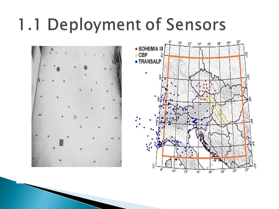
Wireless Sensor Network has millions of nodes, deployed over the wide region for sensing various parameters. As these nodes are deployed in area where human access is difficult, they rely on battery power for functioning. The main purpose of sensor networks is to monitor, combine, analyze and respond to the data collected by hundreds (thousands) sensors distributed in the physical world in a timely manner.
 sensors distributed in the physical world in a timely manner..")
5
The level of activity of node, i.e. transmission reception and processing of data, affects the energy available for the node. If the level of activity is high then battery drains over quickly and that node dies. Hence the network can’t receive any information from that node which is a crucial one in determining the parameter.

6
Also, base stations are highly prone to receive corrupted data from sensors due to noisy wireless environment. As we have many nodes deployed in a region, it is possible to predict the a node’s data neighbors. Also we can predict the value of susceptible node from its past behavior i.e., its data correlation with neighboring nodes for a given condition. Our project deals with these issues.

7
For finding the values of failed sensor nodes various machine learning algorithms can be used as follows: 1. Linear Regression (Not suitable) Collects data values from all sensors. 2. 1-Nearest Neighbor Algorithm (Okay in worst case!) Prediction will be based on only one neighbor, which might not be reliable. 3. K -Nearest Neighbor Algorithm (Best option) Parameters obtained for the failed node will have the influence of nearest k-neighbors, which will minimize the noise.
 Collects data values from all sensors Nearest Neighbor Algorithm (Okay in worst case!) Prediction will be based on only one neighbor, which might not be reliable. 3. K -Nearest Neighbor Algorithm (Best option) Parameters obtained for the failed node will have the influence of nearest k-neighbors, which will minimize the noise..")
8
4 Experiments

10
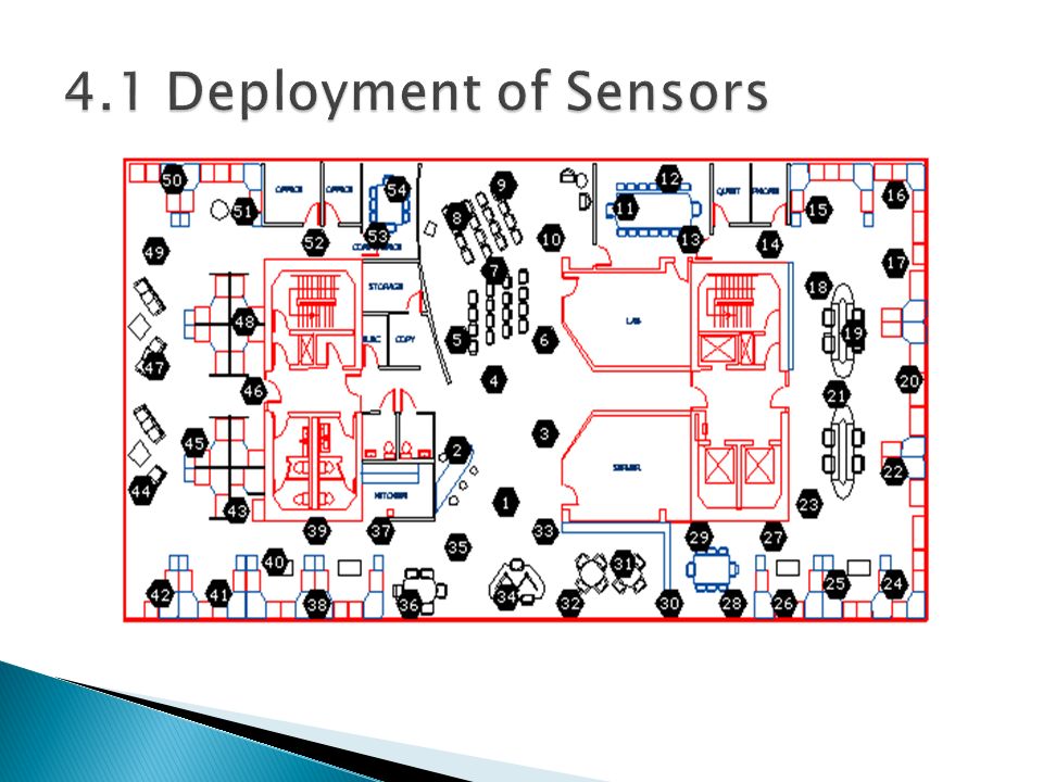
Obtain the co-ordinates of all the sensor nodes physically distributed in the network. Select a node and the time (test instance in ML terms) randomly as susceptible node. Calculate the Euclidean distance of all sensor nodes from the susceptible node. Sorted the distance values and determined Kth nearest neighbor’s distance. Determine K-nearest neighbors. Extract the values of these k-nearest neighbors for the time interval of query time+/-30 seconds and query time-60 seconds. Determine arithmetic mean of these values which is the predicted of the query instance.
 randomly as susceptible node. Calculate the Euclidean distance of all sensor nodes from the susceptible node. Sorted the distance values and determined Kth nearest neighbor’s distance. Determine K-nearest neighbors. Extract the values of these k-nearest neighbors for the time interval of query time+/-30 seconds and query time-60 seconds. Determine arithmetic mean of these values which is the predicted of the query instance..")
12
When Time:3990 and Node ID:41 Output when k is: 2 18.334650,39.704775,326.600000,2.675345 Output when k is: 3 18.109250,40.452563,370.760000,2.678372 Correct value is: 18.1852,39.6878,382.72,2.67532

13
Initialize weight vector to zero Each time test node is encountered in the record, find the difference between the test node’s value and average value of its neighbors at that time and update the weight vector. With the neighbors value at query time and weight vector, test node’s values at query time can be predicted.

14
For implementation based on past history: System gave output for 68% instances with the accuracy of 61.84% For K-NN based implementation when K=2 System gave output for 84% instances with the accuracy of 91.65% K-NN performs better.

16
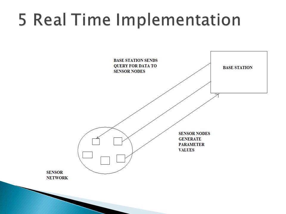
Base station sends request to the sensor network. Parameter values generated by the sensor node. Validity of the values checked by the base station.

17
Sensor nodes are queried for parameter values. If values are missing or null then that sensor node is termed as faulty. When count of occurrence of that faulty sensor node exceeds a particular limit that node is declared to have failed Values from that node not considered in future iterations

18
Automatically generating values from a node. Case when stream of data keeps coming in at that particular sensor node.

19
Parameter values considered at current time interval +- one minute give better accuracy than past history. K-nearest neighbor gives better results than correlation. Cross validation is not considered in our study as it does not improve learning rate of the system.

20
“Protocols and Architectures for Wireless Sensor Networks”, Holger Karl, Andreas Willig, published by Wiley, 2005. “Wireless Sensor Networks”, Raghavendra, Cauligi S.; Sivalingam, Krishna M.; Znati, Taieb (Eds.) 1st ed. 2004. http://www.cs.cmu.edu/~guestrin/Class/10701/projects.html http://www- 2.cs.cmu.edu/~guestrin/Publications/IPSN2004/ipsn2004.pdf http://www- 2.cs.cmu.edu/~guestrin/Publications/VLDB04/vldb04.pdf
 1st ed 2.cs.cmu.edu/~guestrin/Publications/IPSN2004/ipsn2004.pdf 2.cs.cmu.edu/~guestrin/Publications/VLDB04/vldb04.pdf.")
21
Thank You

22
Questions?

Similar presentations