Download presentation
Presentation is loading. Please wait.

1
Atomic Physics with Supercomputers. Darío M. Mitnik

2
Electron-Ion scattering calculations. Darío M. Mitnik

3
Atomic Physics with Supercomputers. Darío M. Mitnik

4
M. S. Pindzola, F. Robicheaux, J. Colgan, Auburn University, Auburn, AL D. C. Griffin, Rollins College, Winter Park, FL N. R. Badnell Strathclyde University, Glasgow, UK

5
Outline What are we calculating? Why do we need supercomputers for such calculations? How do we use the supercomputers in these calculations?

6
What are we calculating? Rate Coefficients Cross Sections

7
Electron-Impact Excitation kiki N electron ion kfkf E th bb aa

8
Electron-Impact Excitation aa bb ii ff

9
(N 1) – electron ion kfkf keke Electron-Impact Ionization kiki EIEI N – electron ion aa
 – electron ion kfkf keke Electron-Impact Ionization kiki EIEI N – electron ion aa")
10
Electron-Impact Ionization aa ee ii ff

11
Radiative Recombination N – electron ion EIEI (N+1) – electron ion kiki aa bb
 – electron ion kiki aa bb")
12
Radiative Recombination M ba = bb a+ ia+ i Photoionization: Radiative Recombination: M ab = 4 2 c 2 /( 2 k i ) |M ba | 2
 |M ba | 2")
13
Dielectronic Recombination M ba = bb a+ ia+ i Photoionization: bb a+ ia+ i nn nn + n + i n /2 +

14
N – electron ion bb EIEI (N+1) – electron ion Dielectronic Recombination kiki nn aa
 – electron ion Dielectronic Recombination kiki nn aa")
15
EIEI 1s 2 2s 1s 2 2s 2 Li-like Be-like 1s 2 2p 1s 2 2pnl 1s 2 2p 3/2 1s 2 2p 3/2 nl

16
Dielectronic Recombination D.M. Mitnik et al, Phys. Rev. A 61, 022705 (2000)
")
17
Dielectronic Recombination D.M. Mitnik et al, Phys. Rev. A 57, 4365 (1998)
")
18
Electron-ion Recombination D.M. Mitnik et al, Phys. Rev. A 59, 3592 (1999)
")
19
Excitation-Autoionization EIEI 1s 2 2s 1s 2 2s 2 Li-like Be-like 1s 2 2p 1s 2 2p 3/2 1s 2 2p 3/2 nl

20
Excitation-Autoionization D.M. Mitnik et al, Phys. Rev. A 53, 3178 (1996)
")
21
Excitation (resonances) EIEI 1s 2 2s 1s 2 2s 2 Li-like Be-like 1s 2 2p 1s 2 2p 3/2 1s 2 2p 3/2 nl
 EIEI 1s 2 2s 1s 2 2s 2 Li-like Be-like 1s 2 2p 1s 2 2p 3/2 1s 2 2p 3/2 nl")
22
Excitation (resonances) D.M. Mitnik et al, Phys. Rev. A 62, 062711 (2000)
 D.M. Mitnik et al, Phys. Rev. A 62, (2000)")
23
Excitation (resonances) D.C. Griffin et al, J. Phys. B 33, 4389 (2000)
 D.C. Griffin et al, J. Phys. B 33, 4389 (2000)")
24
Why supercomputers in Atomic Physics? only a few atomic physicists are using supercomputers

25
“Collisional breakup in a quantum system of three charged particles” M. S. Pindzola and F. Robicheaux, Phys. Rev. A 54, 2142 (1996). Why supercomputers in Atomic Physics? T. R. Rescigno et al., Science 286, 2474 (1999).
. Why supercomputers in Atomic Physics. T. R. Rescigno et al., Science 286, 2474 (1999)..")
26
Electron-Impact Ionization of Hydrogen even the simplest example: e + H H + e + e has resisted solution until now

27
Methods Perturbative methods Non-Perturbative methods Distorted Waves Time-independent Time-dependent

28
Time-independent: R-matrix method P. G. Burke and K. A. Berrington 27 key papers reprinted Short Bibliography list: 547 references

29
Time-independent: R-matrix method Internal RegionExternal Region a Target H = E ~ sin(kr) + Kcos(kr)
 + Kcos(kr)")
30
Why supercomputers? Size of (N+1)-Hamiltonian : MXMAT = MZCHF x MZNR2 + MZNC2 # scattering channels # of continuum orbitals for given L # (N+1) terms for given SL 158 x 50 + 100 = 8000 ~ 512 Mb
-Hamiltonian : MXMAT = MZCHF x MZNR2 + MZNC2 # scattering channels # of continuum orbitals for given L # (N+1) terms for given SL 158 x = 8000 ~ 512 Mb.")
31
Why supercomputers? Thousands of points are needed in order to map the narrow resonances. Energy (eV) Collision Strength D.C. Griffin et al, J. Phys. B 33, 4389 (2000)
 Collision Strength D.C. Griffin et al, J. Phys. B 33, 4389 (2000).")
32
Time-Dependent method Time-dependent Schrodinger equation:

33
Time-Dependent method Time-dependent close-coupled equation:

34
Why supercomputers? 16 x 250 x 250 = 1000000 250 x 250 = 62500 # coupled channels # partial waves # points in spatial lattice

35
Why supercomputers? Memory Time

36
What is a supercomputer? Distributed-Memory Shared-Memory

37
Glossary functional parallelism parallelization data parallelism

38
Example of data parallelism we have 10000 cards we want to pick up the highest card each comparison takes 1 second

39
Example of data parallelism 1 processor 10000 1 sec Time (sec) Processors 2 processors 5000 1 1 sec 10 processors 1008 sec 100 processors 198 sec 10000 processors 10000 sec
 Processors 2 processors 5000 1 1 sec 10 processors 1008 sec 100 processors 198 sec processors sec")
40
Example of a simple program print*, ‘hello world’ stop end call mpi_init call mpi_ rank(iam,nproc) print*, ‘hello world, from process # ’,iam call mpi_finalize stop end
 print*, ‘hello world, from process # ’,iam call mpi_finalize stop end")
41
Example of a simple program hello world hello world, from process 2 hello world, from process 0 hello world, from process 4 hello world, from process 1 hello world, from process 3

42
The R-matrix I package Inner-Region STG1 : calculates the orbital basis and all radial integrals STG2 : calculates LS-coupling matrix elements. solves the N-electron problem. sets the (N+1)-electron Hamiltonian STG3 : diagonalizes the (N+1)-electron Hamiltonian in the continuum basis
-electron Hamiltonian STG3 : diagonalizes the (N+1)-electron Hamiltonian in the continuum basis.")
43
The R-matrix I package Outer-Region STGF : solves the external-region coupled equations. STGICF : calculates level-to-level collision strengths by doing an intermediate- coupling frame transformation.

44
Diagonalization Timing

45
Example 191 x 34 + 506 = 7000 62-state calculation: 191 coupled channels 34 continuum-box orbitals 506 (N+1)-electron bound configurations 55-state calculation (Dell 603): 59 h and 41 min 62-state calculation (T3E-900) : 64-processors - 69 min.
-electron bound configurations 55-state calculation (Dell 603): 59 h and 41 min 62-state calculation (T3E-900) : 64-processors - 69 min.")
46
Parallelization of the external-region codes processor 1 processor 6

47
Time-Dependent method Time evolution of a single-channel: Time-dependent Schrodinger equation:

48
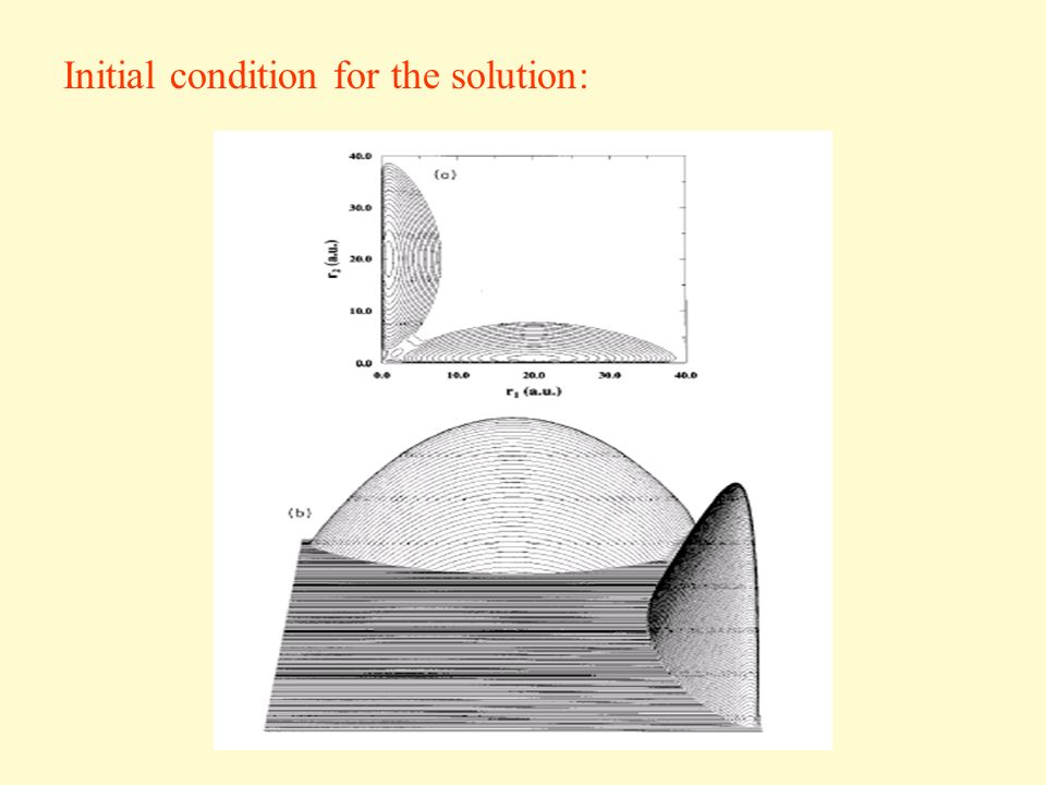
Time-Dependent method Initial condition for the solution:

50
Time-Dependent method

51
Propagated wavefunction:

52
Time-Dependent method Cross Section: Projection of the wavefunction:

53
Parallelization of the time-dependent codes processor 1 processor 6

54
Conclusions Atomic Physics is still alive

Similar presentations


 Klaus Bartschat.>")
 problem we compute ion wavefunctions first, independently.>")


 F. Robicheaux Auburn University Mitch Pindzola and Stuart Loch I.Physical Effects II.Atomic.>")

 Tunneling is one of the simplest quantum mechanical process A Laser STM for Molecules Tunneling has transformed surface science. Scanning.>")


 T. Egami 1, K. Ogata 1, Y. Iseri 2, M. Yahiro.>")


