1. STA617 Advanced Categorical Data Analysis
Instructor: Changxing Ma Department of Biostatistics Kimball, University at Buffalo Phone: (716)
Days, Time: M W, 9:00 AM - 10:20 AM Dates: 08/31/ /11/ Room: Kimbal 126
Office Hours: Monday and Wednesday 10:30-11:30 in RM716 Kimball, or by appointment.

2. STA617 Course Homepage: http://www.acsu.buffalo.edu/~cxma/STA617/
Text: Categorical Data Analysis by Alan Agresti (Second Edition, 2002, Wiley, or new edition) Homepage from the author:
Content: Log linear model, models for matched pairs, analyzing repeated categorical response data, and generalized linear mixed models. We will cover Chapter 8-12 of the textbook.
Computing: SAS

3. Grading
total 300 points: Homework: 100 points Project1: 50 points Project2 or Midterm: 50 points Final project/presentation: 100 points.
5 homework sets, each 25 points, the top 4 scores will be in final homework grade.

4. Date
Event
Monday, August 31, 2015
Classes Begin
Monday, September 7, 2014
Labor Day Observed
Wednesday, November 25 - Saturday, November 28, 2014
Fall Recess
Friday, December 11, 2014
Last Day of Classes

5. Outline of Topics:
PART I – Chp7, Chp8 and Chp9 (logistic, loglinear model 8. Loglinear Models for Contingency Tables 8.1 Loglinear Models for Two-Way Tables 8.2 Loglinear Models for Independence and Interaction in Three-Way Tables 8.3 Inference for Loglinear Models 8.4 Loglinear Models for Higher Dimensions 8.5 The Loglinear_Logit Model Connection 8.6 Loglinear Model Fitting: Likelihood Equations and Asymptotic Distributions 8.7 Loglinear Model Fitting: Iterative Methods and their Application

6. Outline of Topics:
9. Building and Extending Loglinear / Logit Models 9.1 Association Graphs and Collapsibility 9.2 Model Selection and Comparison 9.3 Diagnostics for Checking Models 9.4 Modeling Ordinal Associations

7. Outline of Topics:
Part II: Models for discrete longitudinal data ---matched pairs 10. Models for Matched Pairs 10.1 Comparing Dependent Proportions 10.2 Conditional Logistic Regression for Binary Matched Pairs 10.3 Marginal Models for Square Contingency Tables 10.4 Symmetry, Quasi-symmetry, and Quasiindependence 10.5 Measuring Agreement Between Observers 10.6 Bradley-Terry Model for Paired Preferences 10.7 Marginal Models and Quasi-symmetry Models for Matched Sets

8. Outline of Topics:
--- marginal modeling, GEE, PROC GLIMMIX 11. Analyzing Repeated Categorical Response Data 11.1 Comparing Marginal Distributions: Multiple Responses 11.2 Marginal Modeling: Maximum Likelihood Approach 11.3 Marginal Modeling: Generalized Estimating Equations Approach 11.4 Quasi-likelihood and Its GEE Multivariate Extension: Details 11.5 Markov Chains: Transitional Modeling

9. Outline of Topics:
---subject-specific models, random-effects models PROC GLMMIX, NLMIXED
12. Random Effects: Generalized Linear Mixed Models for Categorical Responses
12.1 Random Effects Modeling of Clustered Categorical Data
12.2 Binary Responses: Logistic-Normal Model
12.3 Examples of Random Effects Models for Binary Data
12.4 Random Effects Models for Multinomial Data
12.5 Multivariate Random Effects Models for Binary Data
12.6 GLMM Fitting, Inference, and Prediction

10. Chapter 8: Loglinear models for contingency tables

11. Two-Way Contingency Tables and Their Distributions
Table 2.1, a 2X3 contingency table, is from a report on the relationship between aspirin use and heart attacks

12. Aspirin and Myocardial Infarction Example
The study randomly assigned 1360 patients who had already suffered a stroke to an aspirin treatment (one low-dose tablet a day) or to a placebo treatment.
follow-up 3 years

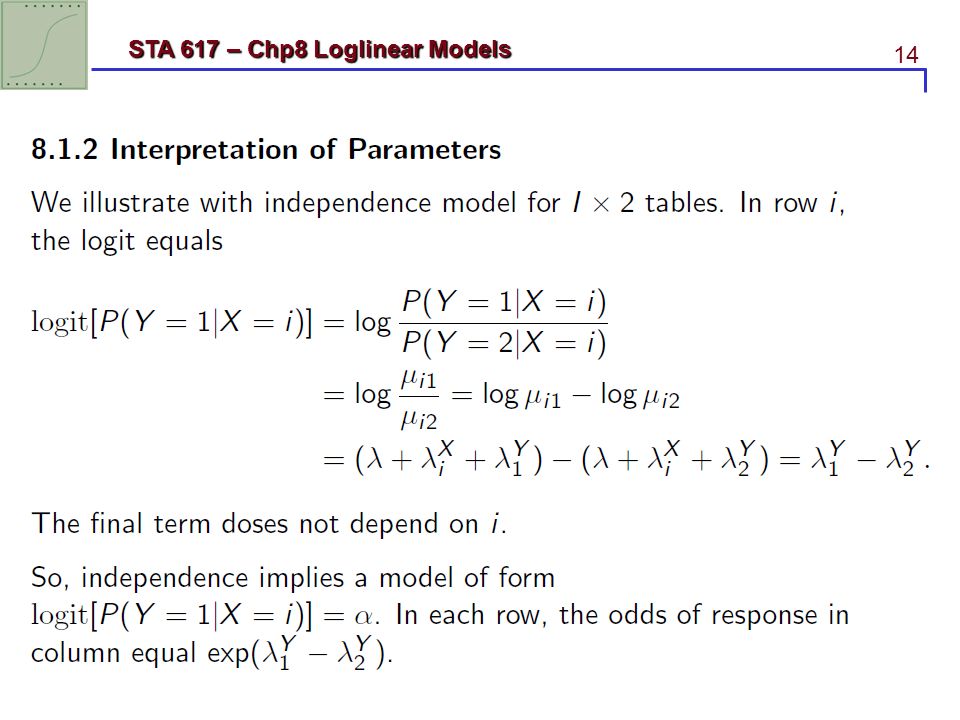
13. 8.1 Loglinear Models for Two-way Tables

16. 8.1.4 Alternative parameter constrains
The estimates are different, but contrasts are unique, such as

17. 8.1.5 Multinomial Models for cell probabilities
The intercept parameter cancels in above formula, because this parameter relates purely to the total sample size, which is random in the Poisson model, but fixed in the multinomial model.

18. 8.2 Logistic Models for independence and Interaction in Three-Way Tables (example)
Table 8.3 refers to a 1992 survey by the Wright State University School of Medicine and United Health Service in Dayton Ohio.
2276 students are asked whether using alcohol, cigarettes, or marijuana in their final year of high school.

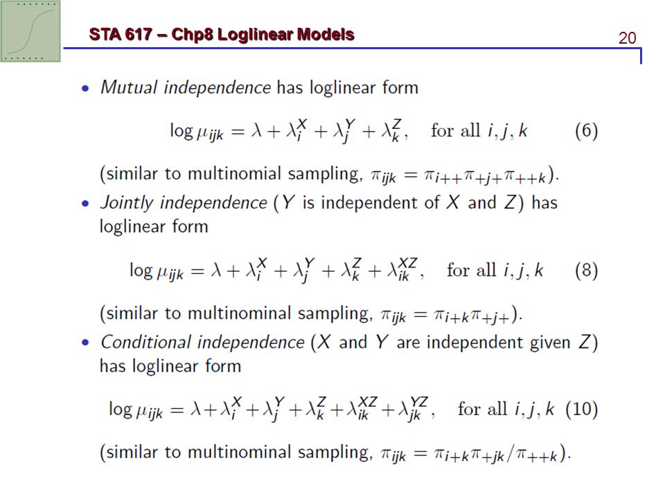
19. 8.2 Logistic Models for independence and Interaction in Three-Way Tables
three-way contingency tables: conditional independence and homogeneous association.
8.2.1 Types of independence
or a multinomial distribution with cell probabilities and
The three variables are mutually independent when (Section 2.3)

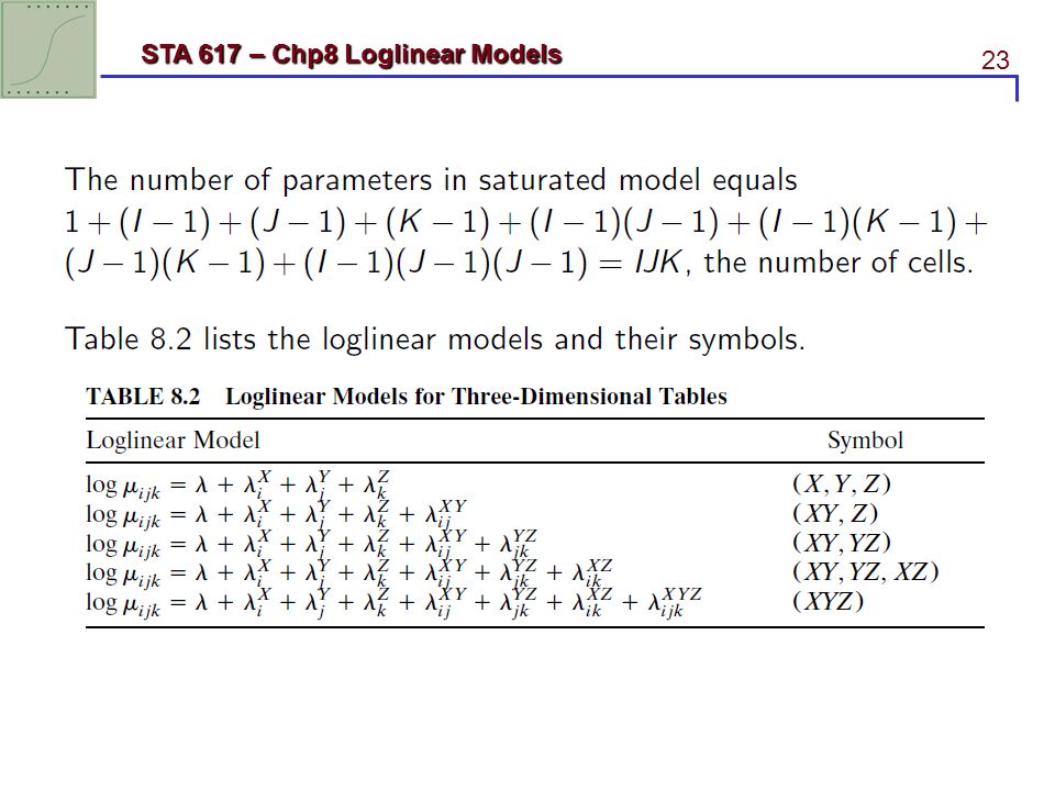
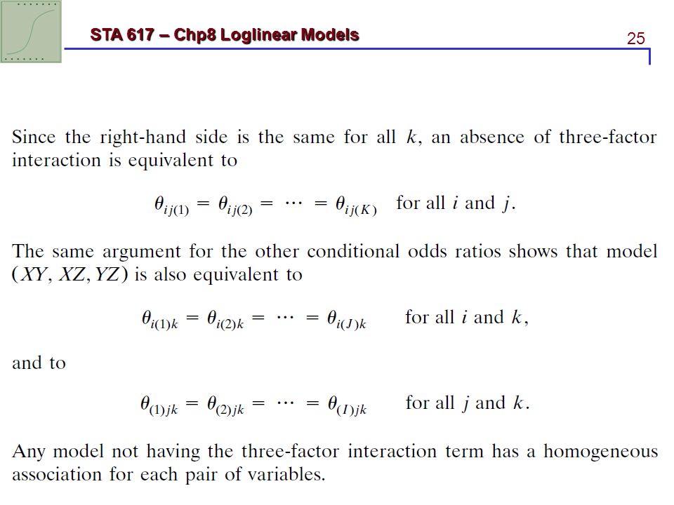
22. 8.2.2 Homogeneous association and three-factor interaction

24. 8.2.3 Interpreting model parameters

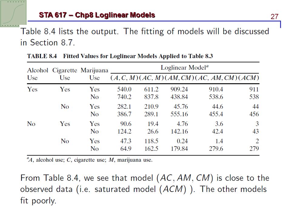
26. 8.2.4 Alcohol, cigarette, and marijuana use example
Table 8.3 refers to a 1992 survey by the Wright State University School of Medicine and United Health Service in Dayton Ohio.
2276 students are asked whether using alcohol, cigarettes, or marijuana in their final year of high school.

28. SAS code
/*data Table 8.3 pp.322*/ data drugs; input a c m count datalines; ; proc genmod data=drugs; class a c m; model count = a c m a*m a*c c*m / dist = poi link = log lrci type3 obstats; ods output obstats=obstats; run;

30. %macro modelbuild(model, varmodel);
proc genmod data=drugs; class a c m;
model count = a c m &model / dist = poi link = log lrci type3 obstats;
ods output obstats=obstats;
run;
data obstats&varmodel; set obstats (rename=(Pred=&varmodel));
label &varmodel=Predicted &varmodel;
keep a c m count Observation &varmodel; run;
%mend;
%modelbuild(, A_C_M);
%modelbuild(A*C, AC_M);
%modelbuild(A*M C*M, AM_CM);
%modelbuild(A*C A*M C*M, AC_AM_CM);
%modelbuild(A*C A*M C*M A*C*M, ACM);
data all; merge obstatsA_C_M obstatsAC_M obstatsAM_CM obstatsAC_AM_CM obstatsACM; by Observation; run;

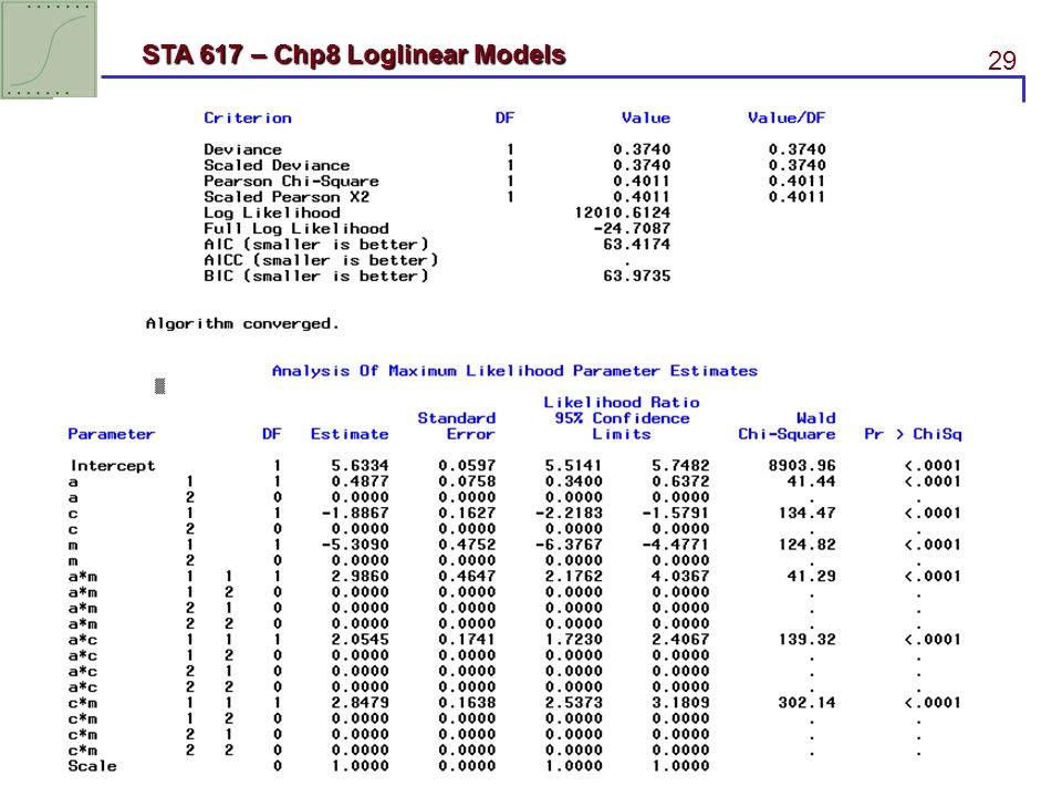
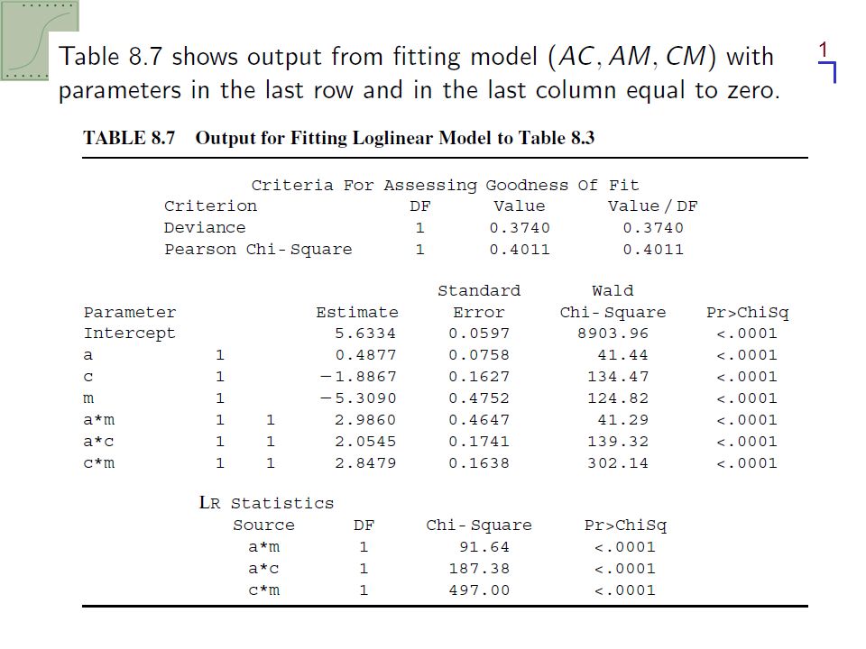
31. SAS output

34. 8.3 Inference for Loglinear Models
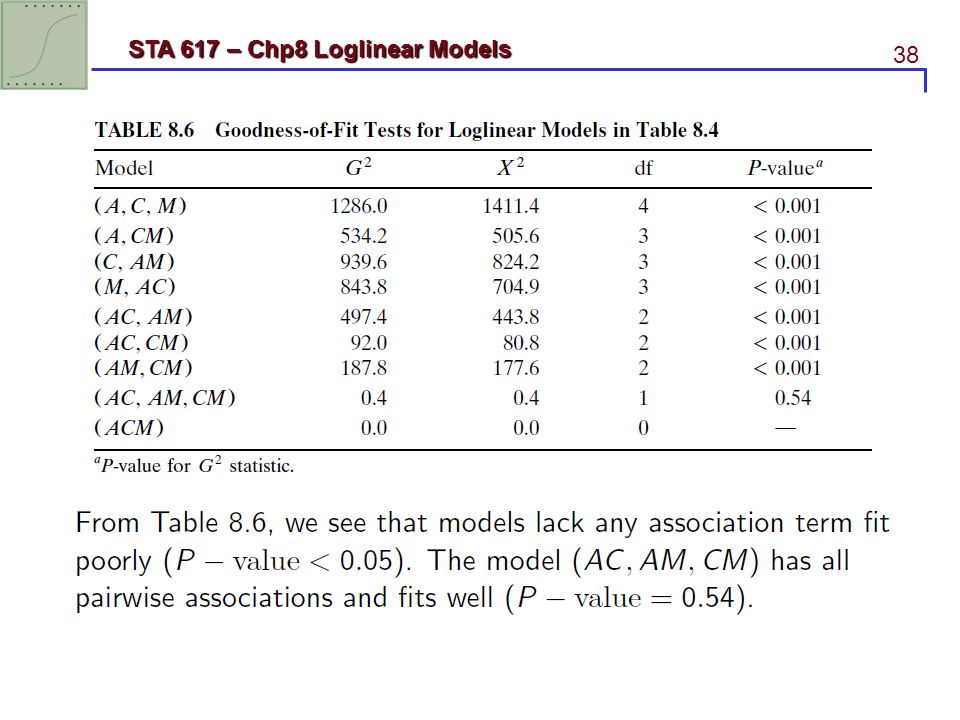
8.3.1 Chi-squared goodness-of-fit tests
As usual, X2 and G2 test whether a model holds by comparing cell fitted values and observed counts. The df equals to the number of cells minus the number of model parameters. df = N − p.
Table 8.6 shows results of testing fit for several loglinear models for the students survey data (see Table 8.3).

35. %macro modelbuild(model, varmodel); proc genmod data=&data; class &maineffect; model count = &maineffect &model / dist = poi link = log lrci type3 obstats; ods output obstats=obstats Modelfit=Modelfit; run; data obstats&varmodel; set obstats (rename=(Pred=&varmodel)); label &varmodel=Predicted &varmodel; keep a c m count Observation &varmodel; run; data _NULL_; set Modelfit; if Criterion='Deviance' then call symput('G2', Value); if Criterion='Scaled Pearson X2' then do; call symput('chi2', Value); call symput('df',DF);end; data newfit; length model $ 50; model="&varmodel"; G2=&G2; chi2=&chi2; DF=&DF; run; data allfit; set allfit newfit; run; %mend;

36. %let maineffect=a c m; %let data=drugs; data allfit; run; %modelbuild(, A_C_M); %modelbuild(C*M, A_CM); %modelbuild(A*M, C_AM); %modelbuild(A*C, M_AC); %modelbuild(A*C A*M, AC_AM); %modelbuild(A*C C*M, AC_CM); %modelbuild(A*M C*M, AM_CM); %modelbuild(A*C A*M C*M, AC_AM_CM); %modelbuild(A*C A*M C*M A*C*M, ACM); data allfit; set allfit; pvalue=1-CDF('CHISQUARE', G2, DF); run; /*Table 8.6 pp.324*/ proc print data=allfit; run;

37. SAS output

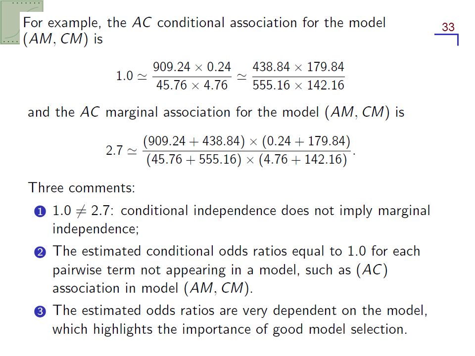
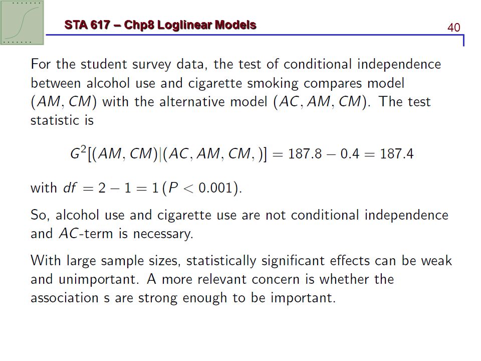
39. 8.3.2 Inference about conditional association

43. 8.4 LOGLINEAR MODELS FOR HIGHER DIMENSIONS
Loglinear models for three-way tables extend to multiway tables.
As the number of dimensions increases, some complications arise.
One is the increase in the number of possible association and interaction terms, making model selection more difficult.
Another is the increase in number of cells. In Section 9.8 we show that this can cause difficulties with existence of estimates and appropriateness of asymptotic theory.

44. 8.4.1 Four-Way Contingency Tables
Four-way table: W, X, Y, and Z
denoted by (WX,WY,WZ, XY, XZ, YZ).
Each pair of variables is conditionally dependent, with the same odds ratios at each combination of categories of the other two variables.
An absence of a two-factor term implies conditional independence, given the other two variables.

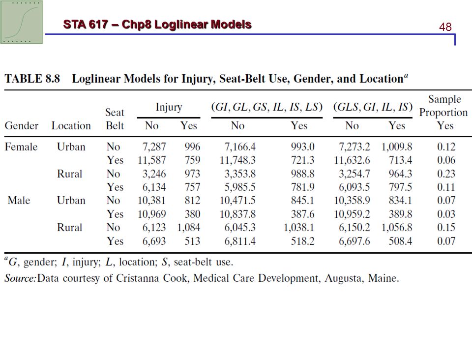
45. 8.4.2 Automobile Accident Example
68,694 passengers in autos and light trucks involved in accidents in the state of Maine in 1991
Variables: gender G, location of accident L, seat-belt use S, and injury I

46. /*table 8.8 pp.327*/
data autoaccident;
input G $ L $ S $ x1 x2;
I="No "; count=x1; output;
I="Yes"; count=x2; output;
drop x1 x2;
datalines;
Female Urban No
Female Urban Yes
Female Rural No
Female Rural Yes
Male Urban No
Male Urban Yes
Male Rural No
Male Rural Yes ;
%let maineffect=G L S I; %let data=autoaccident;
%modelbuild(G*I G*L G*S I*L I*S L*S, I_GL_GS_IL_IS_LS);
%modelbuild(G*L*S G*L G*S L*S G*I I*L I*S, GLS_GI_IL_IS);
data all; merge obstatsGI_GL_GS_IL_IS_LS obstatsGLS_GI_IL_IS;
by Observation;
run;
/*Table 8.8 pp.327*/
proc print data=all; run;

47. SAS output

49. data allfit; run; %modelbuild(, model1); %modelbuild(G. I G. L G. S I
data allfit; run; %modelbuild(, model1); %modelbuild(G*I G*L G*S I*L I*S L*S, model2); %modelbuild(G|I|L G|I|S G|L|S I|L|S, model3); %modelbuild(G|I|L G*S I*S L*S, model4); %modelbuild(G|I|S G*L I*L L*S, model5); %modelbuild(G|L|S G*I I*L I*S, model6); %modelbuild(I|L|S G*I G*L G*S, model7); data allfit; set allfit; pvalue=1-CDF('CHISQUARE', G2, DF); run; /*Table 8.9 pp.327*/ proc print data=allfit; run;

50. Loglinear model fits
SAS:

51. Model1: main effect model (mutual independence) fits very poor (G2=2792.8 P=0)
Model2: main effect+2fis model (homogeneous association) fits still poor (G2=23.4 P<.001), pairwise associations
Model3: main effect+2fis+3fis model (GIL, GIS, GLS, ILS) fits well (G2=1.3, df=1). but is complex and difficult to interpret.
We need find a model more complex than (GI, GL, GS, IL, IS, LS) but simpler than (GIL,GIS, GLS, ILS): model 4-7
Interpretations are more complex for models containing three-factor interaction terms. Table 8.9 shows results of adding a single three-factor term to model (GI, GL, GS, IL, IS, LS).
Of the four possible models, (GLS, GI, IL, IS) appears to fit best.

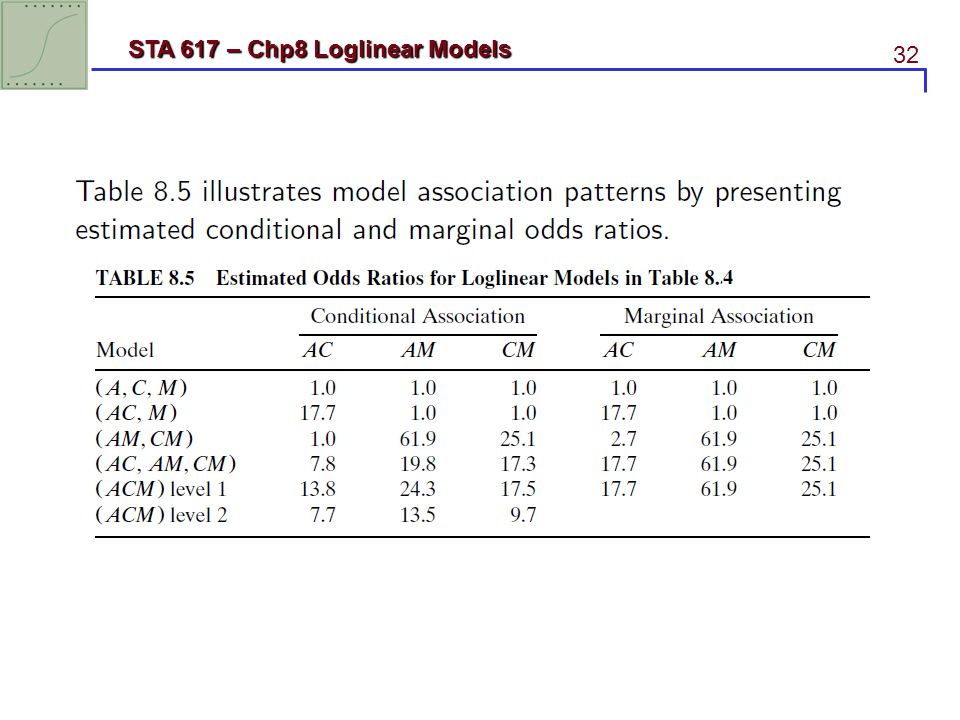
52. Estimated Conditional Odds Ratios
One can obtain them directly using the fitted values for partial tables relating two variables at any combination of levels of the other two.
They also follow directly from parameter estimates; for instance, =exp(-0.814)
95% CI= exp[-0.8141.96(0.0276)] or (0.42, 0.47)
odds of injury for passengers wearing seat belts were less than half the odds for passengers not wearing them, at each gender-location combination.

53. Based on above models

54. The fitted odds ratios in Table 8
The fitted odds ratios in Table 8.10 also suggest that other factors being fixed, injury was more likely in rural than urban accidents and more likely for females than for males.
The estimated odds that males used seat belts were only 0.63 times the estimated odds for females.
For model (GLS, GI, IL, IS), each pair of variables is conditionally dependent, and at each category of I the association between any two of the others varies across categories of the remaining variable.
For this model, it is inappropriate to interpret the GL, GS, and LS two-factor terms on their own. Since I does not occur in a three-factor interaction, the conditional odds ratio between I and each variable (see the top portion of Table 8.10) is the same at each combination of categories of the other two variables.

55. The bottom portion of Table 8
The bottom portion of Table 8.10 illustrates this for model (GLS, GI, IL, IS).
For instance, the fitted GS odds ratio of 0.66 for L=surban refers to four fitted values for urban accidents, both the four with (injury=no) and the four with (injury=yes);
for example

56. 8.4.3 Large Samples and Statistical versus Practical Significance

57. 8.4.4 Dissimilarity Index
This index falls between 0 and 1, with smaller values representing a better fit.
It represents the proportion of sample cases that must move to different cells for the model to fit perfectly.
When the sample data follow the model pattern quite closely, even though the model is not perfect.
For either model, moving less than 1% of the data yields a perfect fit.

58. 8.5 Loglinear-Logit Model Connection

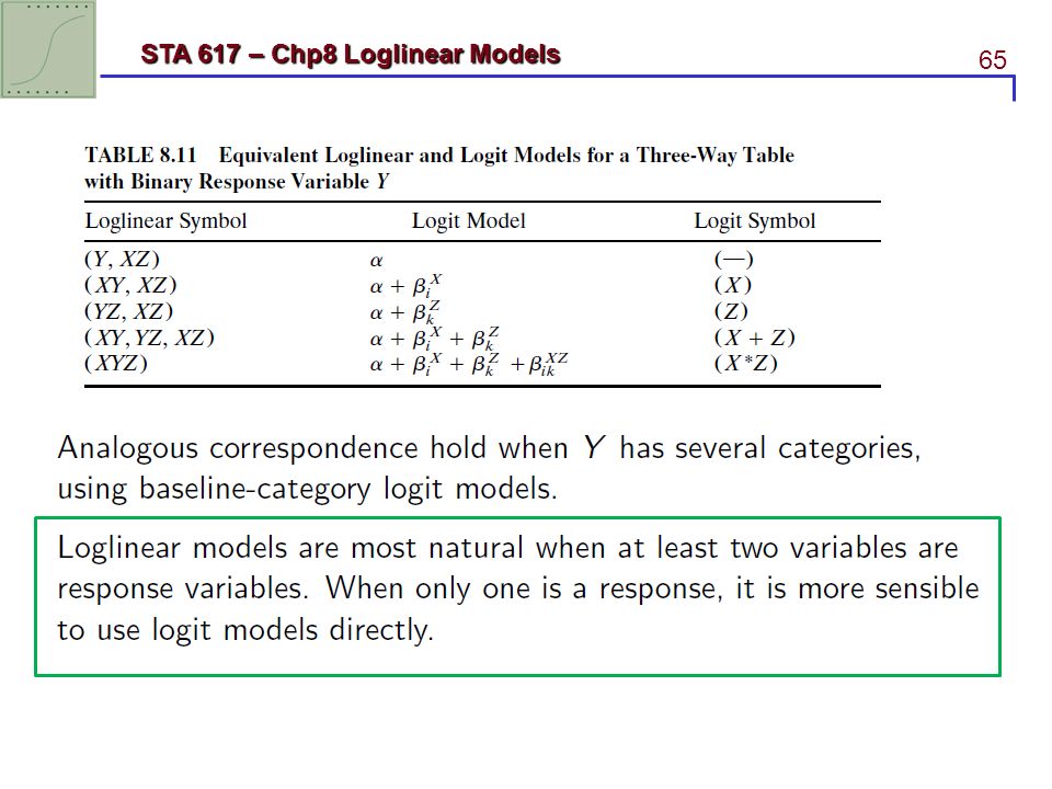
59. 8.5.1 Using logit models to interpret loglinear models

60. 8.5.2 Auto Accident Examples
loglinear model (GLS, GI, LI, IS)
is equivalent to logit model (G+L+S), where we treat injury (I). as a response variable and gender G, location L, and seat-belt use S as explanatory variables
the seat-belt effects in the two models satisfy similar for others.
all terms in the loglinear model not having the injury dropped.

61. Logit vs. loglinear
Loglinear models are GLMs that treat the 16 cell counts in Table 8.8 as 16 independent Poisson variates.
Logit models are GLMs that treat the table as binomial counts. Logit models with I as the response treat the marginal GLS table as fixed and regard as eight independent binomial variates on that response.
Although the sampling models differ, the results from fits of corresponding models are identical.

62. data autoaccident1; input G $ L $ S $ x1 x2; injure=x1; total=x1+x2; drop x1 x2; datalines; Female Urban No Female Urban Yes Female Rural No Female Rural Yes Male Urban No Male Urban Yes Male Rural No Male Rural Yes ; proc logistic data=autoaccident1; class G L S / param=ref; model injure/total=G L S; run;
SAS code

63. Loglinear model
Logistic model

64. 8.5.3 Corresponding between loglinear and logit models

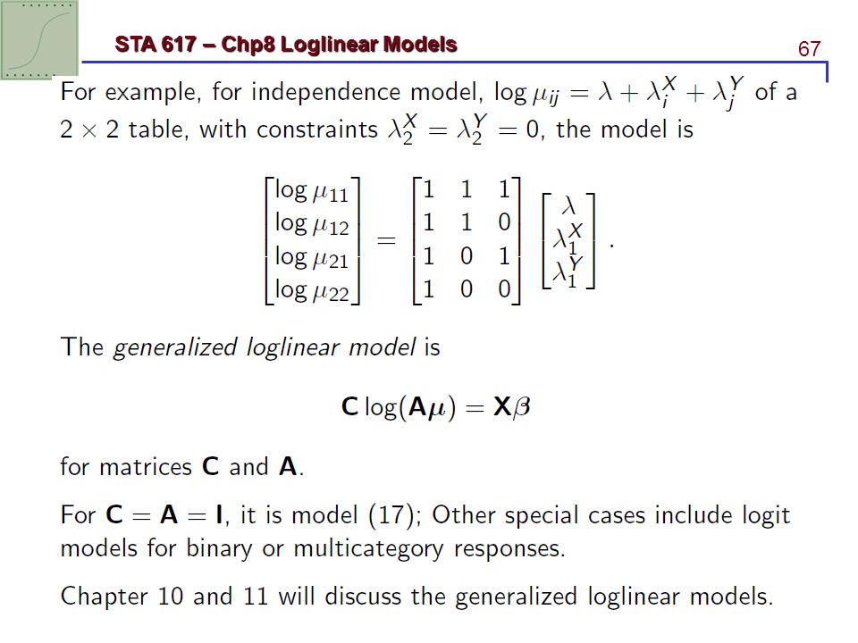
66. 8.5.4 Generalized loglinear model

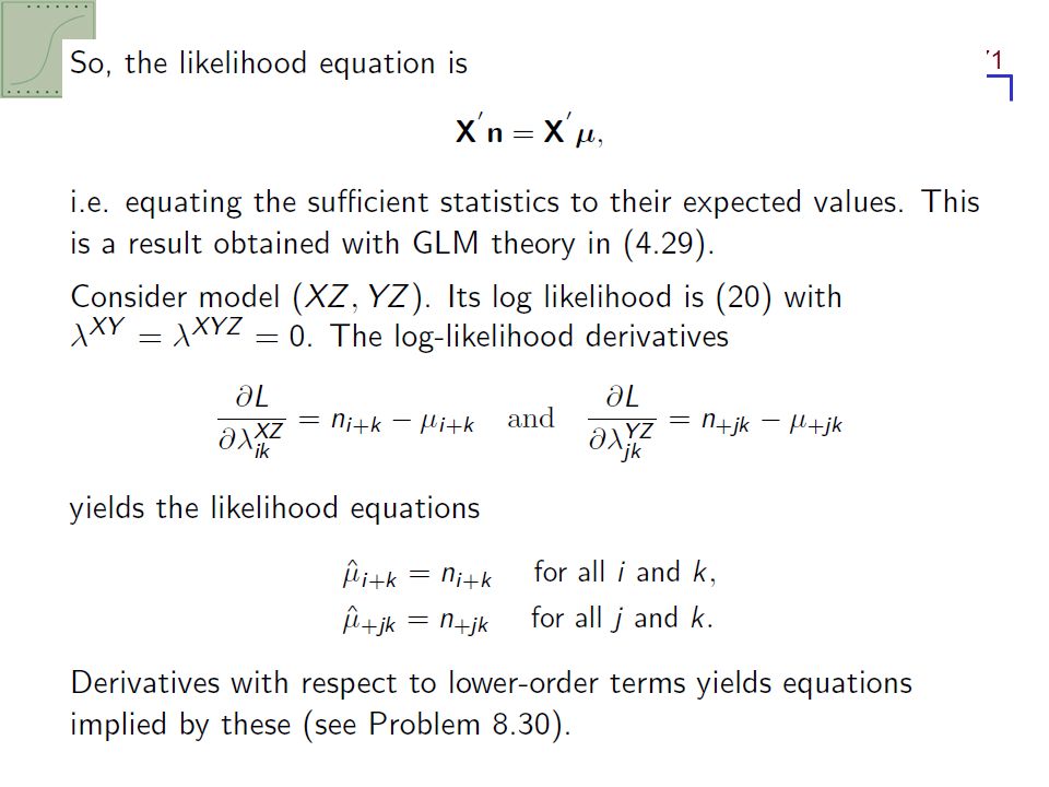
68. 8.6 Loglinear Models Fitting: Likelihood equations and Asymptotic Distributions

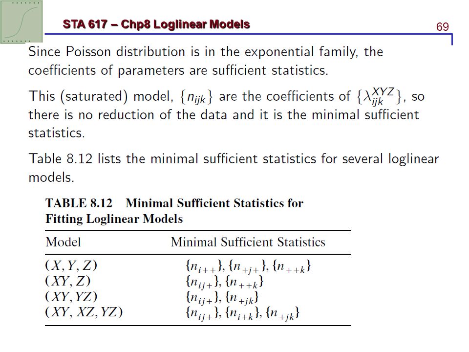
70. 8.6.2 Likelihood equations for loglinear models

73. In practice, it is not essential to know which models have direct estimates.
Iterative methods for models not having direct estimates also apply with models that having direct estimates.
Statistical software for loglinear models uses such iterative methods for all cases.

74. 8.6.5 Chi-squared goodness-of-fit tests

75. 8.6.6 Covariance matrix of ML parameter estimators