1. PARETO POWER LAWS Bridges between microscopic and macroscopic scales

4. Davis [1941] No. 6 of the Cowles Commission for Research in Economics, 1941. No one however, has yet exhibited a stable social order, ancient or modern, which has not followed the Pareto pattern at least approximately. (p. 395) Snyder [1939]: Pareto’s curve is destined to take its place as one of the great generalizations of human knowledge

5. Alfred Lotka the number of authors with n publications in a bibliography is a power law of the form C/n  The exponent  is often close to 1.

6. LOTKA-VOLTERRA LOGISTIC EQUATIONS History, Applications

7. Franco Scudo, "The 'Golden Age' of theoretical ecology. A conceptual appraisal", Rev.Europ.Etud.Social., 22, 11-64 (1984) Franco Scudo e J.R. Ziegler, "The Golden Age of theoretical ecology: 1923-1949", Berlin, Springer, 1978

8. La ricerca ecologica ha avuto, nel periodo 1920-1940, alcuni "anni d'oro", come li ha definiti Franco Scudo (1), con importanti contributi anche italiani (per esempio di V. Volterra e U. D'Ancona).

9. Malthus : autocatalitic proliferation: dX/dt = a X with a =birth rate - death rate exponential solution: X(t) = X(0) e a t contemporary estimations= doubling of the population every 30yrs

10. Verhulst way out of it: dX/dt = a X – c X 2 Solution: exponential ==========  saturation at X= a / c

11. – c X 2 = competition for resources and other the adverse feedback effects  saturation of the population to the value X= a / c For humans data at the time could not discriminate between exponential growth of Malthus and logistic growth of Verhulst But data fit on animal population: sheep in Tasmania: exponential in the first 20 years after their introduction and saturated completely after about half a century.

12. Confirmations of Logistic Dynamics pheasants turtle dove humans world population for the last 2000 yrs and US population for the last 200 yrs, bees colony growth escheria coli cultures, drossofilla in bottles, water flea at various temperatures, lemmings etc.

13. Elliot W Montroll: Social dynamics and quantifying of social forces “almost all the social phenomena, except in their relatively brief abnormal times obey the logistic growth''.

14. - default universal logistic behavior generic to all social systems - concept of sociological force which induces deviations from it Social Applications of the Logistic curve: technological change; innovations diffusion (Rogers) new product diffusion / market penetration (Bass) social change diffusion X = number of people that have already adopted the change and N = the total population dX/dt ~ X(N – X )

15. Sir Ronald Ross  Lotka: generalized the logistic equation to a system of coupled differential equations for malaria in humans and mosquitoes a 11 = spread of the disease from humans to humans minus the percentages of deceased and healed humans a 12 = rate of humans infected by mosquitoes a 112 = saturation (number of humans already infected becomes large one cannot count them among the new infected). The second equation = same effects for the mosquitoes infection

16. X i = the population of species i a i = growth rate of population i in the absence of competition and other species F = interaction with other species: predation competition symbiosis Volterra assumed F =  1 X 1 + ……+  n X n more rigorous  Kolmogorov. Volterra: MPeshel and W Mende The Predator-Prey Model; Do we live in a Volterra World? Springer Verlag, Wien, NY 1986 d X i = X i (a i - c i F ( X 1 …, X n ) )

17. Mikhailov Eigen equations relevant to market economics i = agents that produce a certain kind of commodity Xi = amount of commodity the agent i produces per unit time The net cost to an individual agent of the produced commodity is V i = a i X i a i = specific cost which includes expenditures for raw materials machine depreciation labor payments research etc Price of the commodity on the market is c c (X.,t) =  i a i X i /  i X i

18. The profits of the various agents will then be r i = c (X.,t) X i - a i X i Fraction k of it is invested to expand production at rate d X i = k (c (X.,t) X i - a i X i ) These equations describe the competition between agents in the free market This ecology market analogy was postulated already in Schumpeter and Alchian See also Nelson and Winter Jimenez and Ebeling Silverberg Ebeling and Feistel Jerne Aoki etc account for cooperation: exchange between the agents d X i = k (c (X.,t) X i - a i X i ) +  j a ij X j -  j a ij X i

19. GLV and interpretations

20. w i (t+  ) – w i (t) = r i (t) w i (t) + a w(t) – c(w.,t) w i (t) w(t) is the average of w i (t) over all i ’s at time t a and c(w.,t) are of order  c(w.,t) means c(w 1,..., w N,t) r i (t) = random numbers distributed with the same probability distribution independent of i with a square standard deviation =D of order  One can absorb the average r i (t) in c(w.,t) so =0

21. w i (t+  ) – w i (t) = r i (t) w i (t) + a w(t) – c(w.,t) w i (t) admits a few practical interpretations w i (t) = the individual wealth of the agent i then r i (t) = the random part of the returns that its capital w i (t) produces during the time between t and t+  a = the autocatalytic property of wealth at the social level = the wealth that individuals receive as members of the society in subsidies, services and social benefits. This is the reason it is proportional to the average wealth This term prevents the individual wealth falling below a certain minimum fraction of the average. c(w.,t) parametrizes the general state of the economy: large and positive correspond = boom periods negative =recessions

22. c(w.,t) limits the growth of w(t) to values sustainable for the current conditions and resources external limiting factors: finite amount of resources and money in the economy technological inventions wars, disasters etc internal market effects: competition between investors adverse influence of self bids on prices

23. A different interpretation: a set of companies i = 1, …, N w i (t)= shares prices ~ capitalization of the company i ~ total wealth of all the market shares of the company r i (t) = fluctuations in the market worth of the company ~ relative changes in individual share prices (typically fractions of the nominal share price) aw = correlation between w i and the market index w c(w.,t) usually of the form c w  represents competition Time variations in global resources may lead to lower or higher values of c  increases or decreases in the total w

24. Yet another interpretation: investors herding behavior w i (t)= number of traders adopting a similar investment policy or position. they comprise herd i one assumes that the sizes of these sets vary autocatalytically according to the random factor r i (t) This can be justied by the fact that the visibility and social connections of a herd are proportional to its size aw represents the diffusion of traders between the herds c(w.,t) = popularity of the stock market as a whole competition between various herds in attracting individuals

25. BOLTZMANN POWER LAWS IN GLV

26. Crucial surprising fact as long as the term c(w.,t) and the distribution of the r i (t) ‘s are common for all the i ‘s the Pareto power law P(w i ) ~ w i – 1-  holds and its exponent  is independent on c(w.,t) This an important finding since the i -independence corresponds to the famous market efficiency property in financial markets

27. take the average in both members of w i (t+  ) – w i (t) = r i (t) w i (t) + a w(t) – c(w.,t) w i (t) assuming that in the N =  limit the random fluctuations cancel: w(t+  ) – w(t) = a w(t) – c(w.,t) w (t) It is of a generalized Lotka-Volterra type with quite chaotic behavior x i (t) = w i (t) / w(t)

28. and applying the chain rule for differentials d x i (t): dx i (t) =dw i (t) / w(t) - w i (t) d (1/w) =dw i (t) / w(t) - w i (t) d w(t)/w 2 =[ r i (t) w i (t) + a w(t) – c(w.,t) w i (t)]/ w(t) -w i (t)/w [ a w(t) – c(w.,t) w (t)]/w = r i (t) x i (t) + a – c(w.,t) x i (t) -x i (t) [ a – c(w.,t) ]= crucial cancellation : the system splits into a set of independent linear stochastic differential equations with constant coefficients = ( r i (t) –a ) x i (t) + a

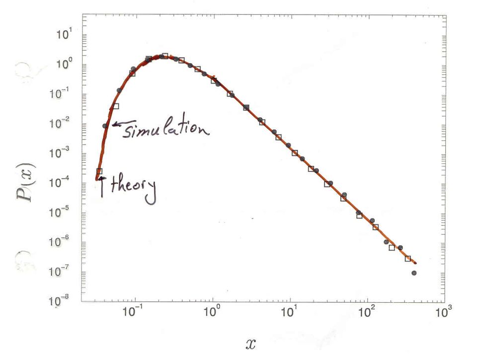
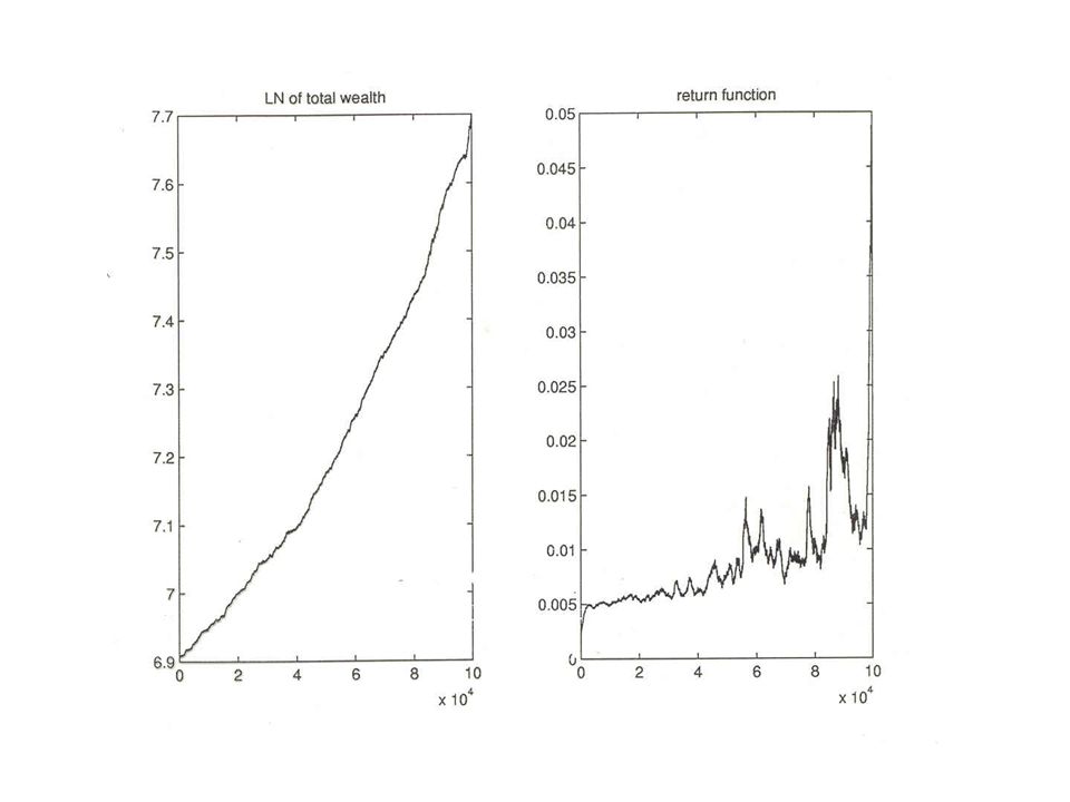
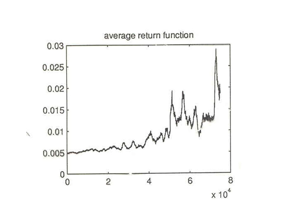
29. dx i (t) = ( r i (t) –a ) x i (t) + a Rescaling in t means rescaling by the same factor in =D and a therefore the stationary asymptotic time distribution P(x i ) depends only on the ratio a/D Moreover, for large enough x i the additive term + a is negligible and the equation reduces formally to the Langevin equation for ln x i (t) d ln x i (t) = ( r i (t) – a ) Where temperature = D/2 and force = - a => Boltzmann distribution P(ln x i ) d ln x i ~ exp(-2 a/D ln x i ) d ln x i ~ x i -1-2 a/D d x i In fact, the exact solution is P( x i ) = exp[-2 a/(D x i )] x i -1-2 a/D

30. 10 0 10 -3 10 -2 10 -1 10 -4 10 -9 10 -4 10 -5 10 -6 10 -7 10 -8 10 -1 10 -2 10 -3 t=0 P(w) w

31. 10 0 10 -3 10 -2 10 -1 10 -4 10 -9 10 -4 10 -5 10 -6 10 -7 10 -8 10 -1 10 -2 10 -3 t=10 000 P(w) w

32. 10 0 10 -3 10 -2 10 -1 10 -4 10 -9 10 -4 10 -5 10 -6 10 -7 10 -8 10 -1 10 -2 10 -3 t=100 000 P(w) w

33. 10 0 10 -3 10 -2 10 -1 10 -4 10 -9 10 -4 10 -5 10 -6 10 -7 10 -8 10 -1 10 -2 10 -3 t=1 000 000 P(w) w

34. 10 0 10 -3 10 -2 10 -1 10 -4 10 -9 10 -4 10 -5 10 -6 10 -7 10 -8 10 -1 10 -2 10 -3 t=30 000 000 P(w) w

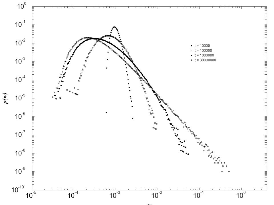
35. 10 0 10 -3 10 -2 10 -1 10 -4 10 -9 10 -4 10 -5 10 -6 10 -7 10 -8 10 -1 10 -2 10 -3 t=0 t=10 000 t=100 000 t=1 000 000 t=30 000 000 P(w) w

39. K= amount of wealth necessary to keep 1 alive If w min revolts L = average number of dependents per average income Their consuming drive the food, lodging, transportation and services prices to values that insure that at each time w mean > KL Yet if w mean < KL they strike and overthrow governments. So c=x min = 1/L Therefore  ~ 1/(1-1/L) ~ L/(L-1) For L = 3 - 4,  ~ 3/2 – 4/3; for internet L  average nr of links/ site

40. In Statistical Mechanics, if not detailed balance  no Boltzmann In Financial Markets, if no efficient market  no Pareto

41. Thermal EquilibriumEfficient Market Further Analogies Boltzmann law One cannot extract energy from systems in thermal equilibrium Except for “Maxwell Demons” with microscopic information By extracting energy from non- equilibrium systems, one brings them closer to equilibrium Irreversibility II Law of Theromdynamics Entropy Pareto Law One cannot gain systematically wealth from efficent markets Except if one has access to detailed private information By exploiting arbitrage opportunities, one eliminates them (makes market efficient) Irreversibility ?

42. Paul Lévy Drawing by Mendes-France

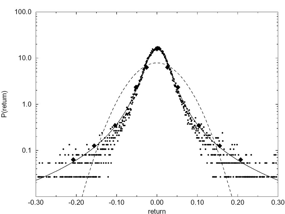
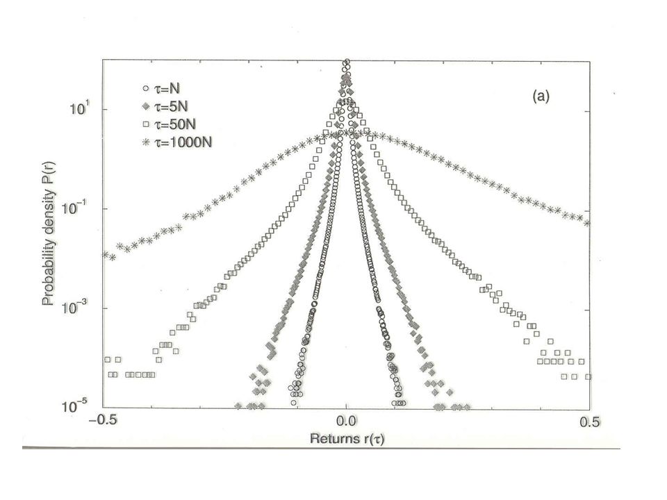
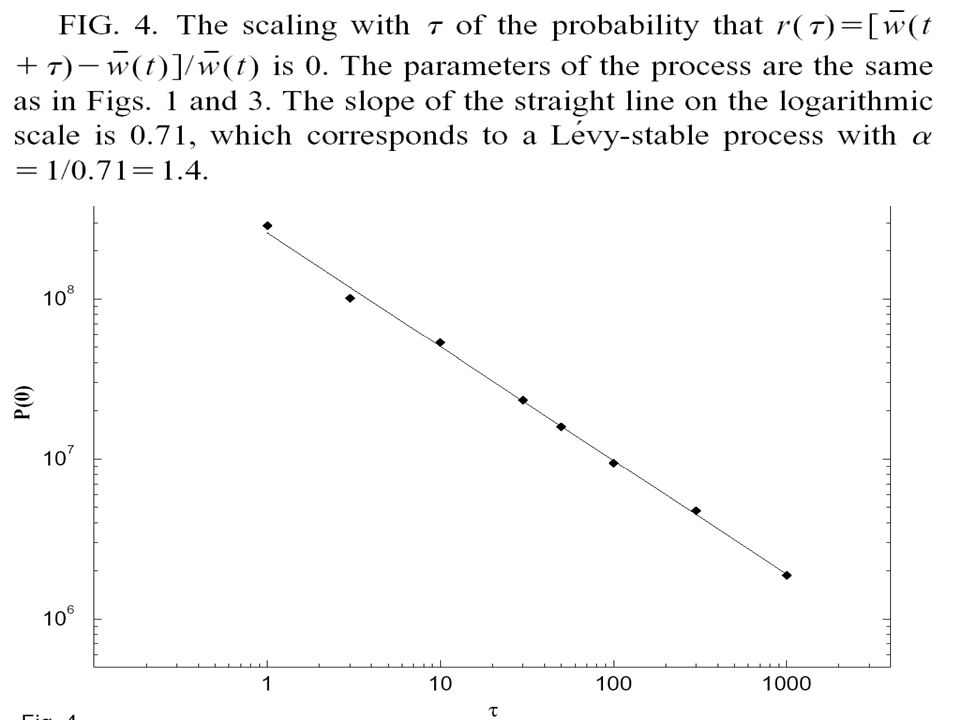
45. Market Fluctuations Scaling

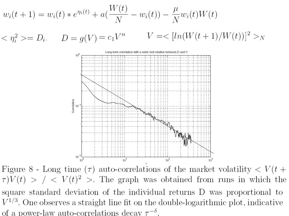
54. Feedback Volatility  Returns => Long range Volatility correlations