1. MECHATRONICS Lecture 07 Slovak University of Technology Faculty of Material Science and Technology in Trnava

2. MECHANICAL VIBRATION

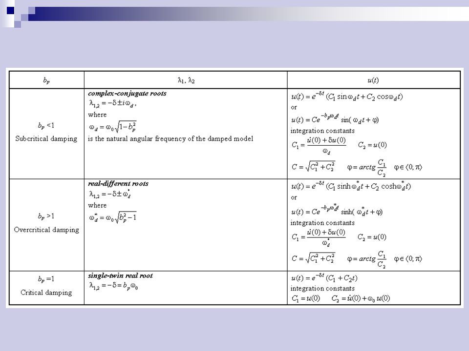
3. Linear model systems Free damped oscillation of the system with single DOF Free oscillation of a damped system is described by the solution of the homogenous equation of motion where m, b, k are parameters of the mass, damping and stiffness, u(t) is the solution (response of the model). The equation can be modified into the form is the decay rate, is the own (natural) angular frequency of the undamped model, is the damping ratio.

4. The solution of the is well known equation where both constants of integration can be solved from the initial conditions for u(0) and ů (0) or from another conditions for u(t) and ů (t) for known time. Values λ 1 and λ 2 are roots of so called characteristic equation:

5. Model and time courses of the linear system with single DOF

7. It is known from the mathematics course that the form of solution for ODR is the sum of homogenous solution and the particular solution. The homogenous solution is valid for F(t) = 0. The form of the particular solution is given by the function F(t). It is obvious from the previous paragraph and Tab. that the homogenous part of the solution disappears after a time. For us the settled damped oscillation (particular part of the solution) is more important and will be analyzed in the following text. Forced damped oscillation of the system with single DOF Excited oscillation of damped system with single DOF is described by the equation or

8. Let us discuss now the case of excitation by a harmonic force with the solution (response, time response) has the form where u 0 is the amplitude of the response, F 0 is the amplitude of the exciting force,  is the oscillating frequence.

9. The absolute value of the expression within the brackets is the transfer function (see also the frequency characteristics) H(ω). Substituting u 0 = F 0 / k - static sag and η = ω/ω 0 - frequency tuning we have The real part is the responce to the exciting force F 0 cos ω t and is equal to where the phase angle φ means the delay of the response to the excitation due to damping of the model system. The amplitude frequency characteristics The phase frequency characteristics

10. The frequency characteristics (i.e. amplitude vs. frequency and phase vs.frequency) for two types of excitation force: Characteristics for harmonic force

11. The excitation by rotating mass Very often the excitation is caused by unbalanced rotating mass. Such case is shown on Fig. The unbalanced rotor is represented by the mass m n placed on the eccentricity r n from the axes of rotation. m is the total mass of the equipment. The resultant stiffness is k and the damping is b. The vertical inertia force is F = m n r n ω 2 sinωt. The equation of motion is When we compare this equation with basic equation for forced vibration, we see that both equation F(t) = m n r n ω 2 sinωt The solution is identical to that excited by harmonic force. The amplitude of sustained vibrations is given by following formula

12. This expression is possible to plot in the amplitude and phase diagram The frequency transfer and the phase frequency characteristics is defined as

13. Exciting force is a periodic function of time In many cases the exiting force is a periodic function of time. It means that its value repeat after the period T F F(t) = F(t+T F ) = F(t+n T F ) for n = 1, 2,..., n In such case it is possible expand the force into Fourier series The equation where  = 2  /T F. The determination of Fourier coefficients is well known from mathematics In practical applications we do´nt take infinity number of Fourier coefficients, but only n.

14. . The right hand side of we arange when used F 1i = F i sin  Fi,F 2i = F i cos  Fi, for i = 1, 2,... So it is Now we can re-write the equation in the form If holds the law of superposition we can determine the response for each component of the force separately and then the resultant response is given by adding all particular calculated responses due to separate harmonic terms.

15. The general solution is obtained again from the homogeneous and particular solutions The amplitude of particular solution is done by In this equation is

16. From we see that, that particular harmonic components magnified the response according the value of F i and the order i. Very often the course of forces is known from measurements. In such case the components of Fourier series is also possible to get from measured values. We consider the period of the force is T F and the number of of measurements is N+1. The time interval will be Δt = T F /N, and the time from the beginning of force action is t j = jΔt. We introduce the value The measured function will be denoted by Y(t j ) = Y j. The coefficients of Fourier series are determined by for i = 1, 2,...

17. The kinematical excitation The exciting, considered so far has been done by the force acting on the moving mass. Now we shall consider that the frame move harmonically according the formula u z (t) = h sinωt. Such case is sometimes called seismic excitation. The differential equation of motion of the moving mass will be It is seen that the motion is harmonic. If we consider that the base move according the function f(t) is f(t) = bhω cosωt + kh sinωt After arrangement of we get

18. Using the notation and the equation obtains the form From here we get By using of these expressions the equation obtains the form The right hand side of is possible to simplify by notation

19. The particular solution of this equation will be. with the amplitude of harmonic motion of the mass The course of frequency transfer λ is shown in Fig. The phase is given by the formulas

20. . Kinematical excitation

21. The force is general function of time Very often the excitation force is a general function of time. The particular solution is given by Duhamel integral: The analytical solution of this integral is possible for simple functions of general force.