1. A unified approach to learning spatial real estate economics Daniel Gat Center for Urban and Regional Studies at the Technion argat@technion.ac.il

2. A Naïve Model of Housing in a Mono-Centric City Begin with some well known assumptions: 1.City in a featureless plain 2.Radial travel only to a single center where everyone works and shops, so location is a single parameter x, the home to work distance 3.No travel congestion so household travel costs T(x) = tau*x, 4.All households are identical and with equal wage y and tastes 5.Tastes are reflected by the household welfare function u whose arguments are (a) housing consumption h, measured in sqm of home area, and (b) all other consumption measured by residual income z after rent and commuting costs (eq. 1)

3. Optimal Consumption Given Cobb Douglas, household-welfare is maximized when housing expenditures and other expenditures respectively equal (eq.2) Let R(x) be the unit rent. Plugging equation (2) into (1) we get But welfare is equal across all households at all locations (assumption 4) including at the center where there are no travel expenses. This yields the rent gradient equation: (eq.3)

4. Housing Consumption and Distance Housing expenditures are (eq. 4) In other words, given income y, travel costs tau and bid rent R(x), optimal housing size (in sqm) grows with distance from the single center, and the function h(x) is convex. What about the consumption of land for housing as a function of distance?

5. Land consumption in the housing production process Floor space F is produced by combining land L (measured in sqms) with non land resources (capital measured in money units) C, according to the function (eq. 5) Where A is the overall productivity. Floor area Ratio FAR is known as the amount of floor space per unit of site area. Using (5): (eq. 6) Equation 5 always holds whether production is optimal or not. Let be the unit price of land. Since resources are sunk in the process of building, the price of building is 1. (At this point, the time to market is ignored, to be re- visited later on).

6. Land consumption in production (continued 2/3) Optimality yields the following results: (eq. 7) Where V is the unit price of the finished floor area. V is related to R through: Where is the capitalization rate. Divide the rows of 7 to get (eq. 8) From (7a) we get (eq. 9)

7. Land consumption in production (continued 3/3) Combining (6) and (8) we get (eq. 10) From (7a): (eq, 11) Combining (9) and (11), we end up after some algebra with lambda star, the optimal unit value of land given that we know V, the value of floor space or its corresponding rent R. (eq.12). We see that is a convex function of V. In fact, since beta is empirically around 1/3, is related to the 3 rd power of V, so that small movements in the price of floor-space can lead to large movements in land value. Hence, probably, one of the reasons real estate development firms are highly volatile. (That is definitely the case in Israel).

8. Optimal Floor Area Ratio FAR* Optimal value of land is of course contingent on building at the optimal FAR whose value can be computed by plugging lambda star back into equation (10) above, thusequation (10) above Which simplifies into (eq. 13). So optimal floor area is roughly related to the square of V. Now we know from equation (3) that rent is negatively related to distance. Therefore, so is the price V: (eq.14)

9. Optimal Land Value and Floor Area Ratio FAR* Related to Distance from CBD By plugging (14) into (2) and (13) we get the expressions for Lambda star an FAR star as functions of x, the distance between home and CBD. (eq. 15) Note that both the distance gradients of the unit value of land and that of the optimal FAR have become considerably steeper. ( in the denominator ). This reflects two trade-offs, that of area for distance by the consumer and that of capital for land by the producer; both trade-offs display diminishing returns to size. Note also use of the general term T(x) and not the specific x times tau. This will be useful soon. End of the Naïve Mono-Centric Model.

10. Interim Conclusions This naïve model even with its crude assumptions is agood first introduction to urban land economics. Although the demand section is about housing, the model is also a launching platform for understanding non-housing land use since any use needs to compete with housing which which in all cities dominates the landscape. The variations which I have developed – but won’t show here – include: Quality of the building and a link to Hedonics Automotive travel congestion and a multi mode city Variety of household types, e.g. “space seekers” and “action seekers” Time to market and the substitution of NPV for profit as the maximand Redevelopment by demolition (optimal and constrained by zoning) Urban quasi-dynamics of a city with long lived but replaceable buildings The variation that I would like to peek at, just to show how far this model will take us is: “Going from Mono to Poly”

11. Going from Mono to Poly The switch is absolutely simple. The only major assumption that needs to be changed is that of a single center. In the poly version a set of centers is defined by specifying size and coordinates of each center. Given a city with several centers entails 3 modifications: (1)Location is no longer a single number x. Instead, it is x = (x 1, x 2 ), a vector of the two coordinates. (2)The consumer now has to decide how to allocate its trips between alternative destinations. We know how to do that – using a discrete choice probability model and then averaging. (3)The result is the expected monthly vehicle miles ensuing from a household at each location (x 1, x 2 ). Multiply by that by the unit cost of travel and we have T(x). Plug T(x) into the rent equation (3) and the others that follow, and we are home free.

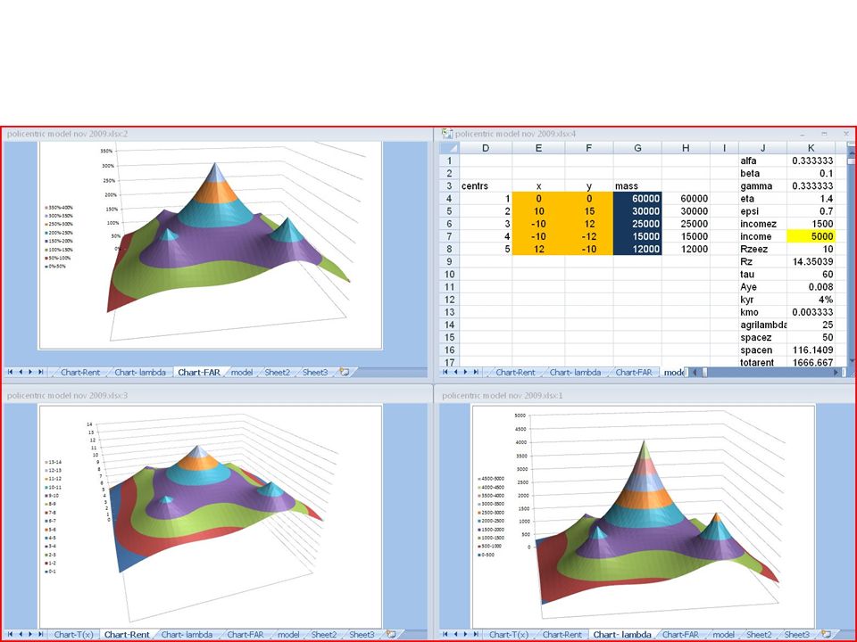
12. Instead of going through the formal equations I will show you some 3 D graphic results of simulating the polycentric model, (rent, land value and optimal FAR when income is set at 3, 4 an 5 k dollars per month) and then compare these results with some figures from the literature.

15. Literature Examples Berry 1963: polycentered chicago commercial structure Alonso 1964: a city model with two centers Romano 1972: a city model with two centers Bernick and Cervero 1997: Bay area employment densities Cervero 1998: Sketch model of adaptive city Redfearn 2006: Semi-parametric model of Krakow