Chapter 4 Minimum Cost Flow Problems (MCF)

Chapter 4 Minimum Cost Flow Problems (MCF)
Network Optimization Chapter 4 Minimum Cost Flow Problems (MCF)

4.1 The upper-bounded transshipment problem
In Chapter 2, we learned uncapacitated transshipment problem, i.e., the flows along the arcs does not have capacity restriction. We now consider capacitated transshipment problem: min cx s.t. Ax=b 0  x  u

The cost vector c and supply/demand vector b are defined as before, u is the capacity vector, i.e., we request xij  uij for each arc (i,j). The capacitated transshipment problem is usually called minimum cost flow problem.

If in addition to the upper bound u, the flows also have (nonzero) lower bound constraint x  v, it is easy to change all lower bound to 0. For example, if we ask xij  vij for each arc (i,j) then we introduce new variables x’ij = xij - vij So, vij xij  uij  0  x’ij uij -vij. Let vector =u - v, then 0 x’  .

A problem is defined as follows : min cx min cx+cv s.t. Ax=b s.t. Ax=b-Av v xu x’ 

Let =b-Av, then the above problem is equivalent to min cx’ s.t. Ax’= 0 x’  So, we can always assume the lower bound v is a 0 vector.

We now extend the network simplex method to solve MCF problems. To do so, we need to recall the simplex method to the LP problems with upper bound constraints in which non-basic variables can have either 0 value (lower bound value), or the upper bound value.

Let x be a feasible flow to the MCF problem min{cxAx=b, 0 xu}. For each arc (i,j), if xij =0, we say (i,j) is free w.r.t. x if xij =uij, we say (i,j) is saturated w.r.t. x if 0< xij <uij, we say (i,j) is unsaturated w.r.t. x

Feasible Tree Solution x (FTS): (1) x is a feasible flow (meet non-negativity, capacity and supply/demand requests). (2) there is a spanning tree T such that any arc not in T is either free, or saturated. In other words, only the arcs in T can be unsaturated arcs.

Dual variables y w.r.t. a FTS x Again, the variables y are determined by the equations yj - yi=cij, (i,j) T and set yn =0.

Profitable arc An arc (i,j)T is called a profitable arc if yj - yi< cij when (i,j) is a free arc, or yj - yi > cij when (i,j) is a saturated arc.

Theorem 4.1 : An FTS x without profitable arcs is an optimal solution. Proof : Let x’ be any feasible solution. We need to show that cxcx’. Let d=c - yA (expressed as a row vector), i.e., dij =cij +yi - yj. cx = (d+yA)x = dx+yb. cx’= (d+yA)x’= dx’+yb. We should compare dx and dx’.

(i) if (i,j) T, then dij = 0  dij xij = dij x’ij. (ii) if (i,j) T and is a free arc. dij 0 (non-profitable), xij = 0, x’ij  0  dij xij  dij x’ij . (iii) if (i,j) T and is a saturated arc, dij  0 (non-profitable), xij =uij x’ij Therefore, dx = dij xij  dij x’ij =dx’  cx  cx’. The proof is completed.

By the above theorem, if x is not optimal, then there is at least one profitable arc, say (p,q). If (p,q) is free and profitable, when xpq increases from 0 to t, the objective function value shall decrease (the reason is similar to the un-capacitated case in Ch.2). If (p,q) is saturated and profitable, then xpq = upq. If we obtain a new FTS x’ with x’pq = upq - t (t>0) and x’ij =xij for other arcs (i,j)T, the objective function value shall decrease. The reason is below.

Let F be the set of free arcs, S be the set of saturated arcs w.r.t. x. Since d = c - yA, cx’ - cx = dx’ - dx. For the value of dx, as dij = 0, (i,j)  T xij = 0, (i,j)  F xij = uij, (i,j)  S we have dx =

For the value of dx’, as x’ij = xij = 0, (i,j)  F x’ij = xij = uij, (i,j) S & (i,j)≠(p,q) x’pq = upq - t we have dx’= = dpqt Therefore, dx’- dx = - dpqt. As (p,q) is profitable, by definition, dpq = cpq + yp - yq > 0. Therefore, dx’ - dx < 0  cx’ < cx.

How to obtain an improved solution:  Adjoin the selected profitable arc e to the spanning tree T to obtain a unique cycle C(e).  The arcs in C which have the same direction as e are forward arcs and otherwise backward arcs.

 If e is free, increase flows on e and each forward arc by t, and reduce flows on each backward arc by t;  If e is saturated, decrease flows in e and each forward arc by t, and increase flows on each backward arc by t. if e is a free arc if e is a saturated arc

 The value of t is determined by the non-negativity and capacity requests, i.e., until the flow along an arc f in T is first reduced to 0, or increased to its upper bound. This arc f is the leaving arc, and the new spanning tree is T’= T + e – f. if e is a free arc if e is a saturated arc

Network simplex method for minimum cost flow problems Step 1. The current FTS is x with a tree T. Any arc not in T is either free or saturated. Step 2. Obtain a (unique) vector y with n components, the last being zero, by solving the n - 1 defining equations of the type yv - yu = cuv, where (u,v) is an arc in T.

Step 3. Let dij = cij + yi - yj. A free arc (i,j) is profitable if dij is negative. A saturated arc (i,j) is profitable if dij is positive. If there are no profitable arcs with respect to the current FTS x, then x is optimal and we stop. Step 4. Otherwise choose a profitable arc e = (p,q) as the entering arc. Then a unique cycle C is created. Arcs in C which have the same direction as e are forward arcs, the others being backward arcs.

Step 5. (a) If the entering arc e is free, then add t units along e and also to the flow along all forward arcs. At the same time subtract t units from the flow in all backward arcs. (b) If the entering arc e is saturated, then subtract t units from the flow in e and also from the flow in all forward arcs. At the same time add t units to the flow in all backward arcs. (c) t is non-negative and the choice of t is subject to capacity constraints and to the non-negativity constraints of the flow vector.

Step 6. Choose t such that in the cycle C there is at least one arc which becomes free or saturated. Remove one such arc, say f, from T, creating a new tree T’=T+e-f and an updated flow x’. Go back to Step 2.

Example 4.1 Suppose in the network below, the supply-demand vector bT = [-9, 4, 17, 1, -5, -8], xT = [x12, x13, x15, x23, x42, x43, x53, x54, x56, x62, x64], cost vector c = [3, 5, 1, 1, 4, 1, 6, 1, 1, 1, 1], capacity vector uT = [2, 10, 10, 6, 8, 9, 9, 10, 6, 7, 8].

For the two numbers beside each arc, for example (3,2) beside e1, the first is cost, & the second is capacity. Suppose we have an initial FTS xT = [2, 0, 7, 5, 0, 9, 3, 3, 6, 7, 7], z = cx =68, with the spanning tree T shown below.

xT = [2, 0, 7, 5, 0, 9, 3, 3, 6, 7, 7] Iteration 1 : Step 1. using the formula yj - yi = cij, (i,j)T we obtain y=[-1,5, 6, 1, 0, 0]. The arc (1,3) is free and d13 = c13 + y1 - y3 = 5 + (-1) –6 = -2 < 0

Step 2. The arc (1,3) is free and d13 = c13 + y1 - y3 = 5 + (-1) –6 = -2 < 0 (1,3) is a profitable arc ~ take it as the entering arc e. x13: 0→t, x53: 3→3-t, x15: 7→7-t

x13: 0→t, x53: 3→3-t, x15: 7→7-t Choose the largest possible t to meet the conditions: t  u13 =10, t  0, t  0  t = 3 (5,3) ~leaving arc. Iteration 2 : Step 1. The new xT=[2, 3, 4, 5, 0, 9, 0, 3, 6, 7, 7], z=62 with the tree T shown below.

xT=[2, 3, 4, 5, 0, 9, 0, 3, 6, 7, 7] y=[-1, 3, 4, 1, 0, 0] The arc (5, 6) is saturated and d56 = c56 + y5 - y6 = – 0 > 0.

Step 2. The arc (5, 6) is saturated and d56 = c56 + y5 - y6 = – 0 > 0. So, (5,6) is profitable ~ take as the entering arc e. x56: 6→6-t, x64: 7→7-t, x54: 3→3+t

x56: 6→6-t, x64: 7→7-t, x54: 3→3+t. Under the condition x56 0, x64  0, x54  u54 = 10, we take t=6 and (5,6) is the leaving arc f. Note that e=f, and hence T does not change, but the iterative solution x is changed.

Iteration 3 : Step 1. xT=[2, 3, 4, 5, 0, 9, 0, 9, 0, 7, 1] with z=56. y=[-1, 3, 4, 1, 0, 0]. (Note that y does not change because T is the same) Step 2. There are no profitable arcs. So, the current FTS is optimal.

4.2 Initialization Just like the un-capacitated case, in order to obtain an initial FTS, we need to locate a vertex v satisfying three properties: 1. If i is a source, then there is an arc from i to v whose capacity is not less than the supply at i. 2. If j is a sink, then there is an arc from v to j whose capacity is not less than the demand at j. 3. If k is an intermediate vertex, then there is an arc from v to k or from k to v.

4.2 Initialization If we cannot find such a vertex v, we choose an arbitrary vertex v and construct artificial arcs if necessary to meet these requirements. The only difference from the un-capacitated case is that if there is an arc from a source to v (or from v to a sink) in the network, but its capacity is less than the supply of the source (or the demand of the sink), then we still need to construct an artificial arc with unlimited capacity from the source to v (or from v to the sink).

4.2 Initialization For example, take vertex 2 as v. Even though there is an arc (3,2) from source 3 to v, as its capacity u32 = 1 < 9 (the supply), we need to introduce another arc (artificial arc) (3,2) with unlimited capacity.

4.2 Initialization After introducing the artificial arcs, we solve an MCF problem with c’ij = If the optimal value is 0, the original MCF problem is feasible and we obtain an FTS, otherwise, the original problem is infeasible.

4.2 Initialization Example 4.2 xT = [x12, x13, x24, x32, x34] capacity vector uT =[8, 3, 16, 1, 8] supply/demand vector bT = [-7, 10, -9, 6] Take vertex 2 as v. We use x’32 to denote the flow along the artificial arc and consider the arc as the last arc.

4.2 Initialization Let c’ = [ ]. We solve the MCF problem. The optimal solution is x12 = 7, x13 = x24 = x32 = 0, x34 = 6, x’32 = 3. Since the optimal value c’x = 3 > 0, the original problem is infeasible. In fact, the flow along the artificial arc is x’32 = 3, which is still positive.

4.2 Initialization Exercise Formulate the following problem as a Minimum-Cost-Flow problem (but you do not need to solve the problem). You may formulate it by simply giving a suitable network in which you specify (cost, capacity) along each arc and the net supply (S) or demand (D) beside some vertices.

4.2 Initialization Oilco has oil fields in San Diego (SD) and Los Angeles (LA). The SD field can produce up to 5 units of unrefined oil (1 unit =100,000 barrels) per day, and the LA field can produce up to 4 units per day. Oil is sent from the fields to a refinery, either in Dallas (DA) or in Houston (HO) (assume each refinery has unlimited capacity). To refine one unit costs＄800 at DA and＄1,000 at HO. Refined oil is shipped to customers in Chicago (CH) and New York (NY). CH customers require 4 units of oil per day, and NY customers require 3 units per day. The costs of shipping one unit of oil (refined or unrefined) between cities are shown in the table below:

4.2 Initialization TO From Dallas Houston New York Chicago Los Angeles
＄300 ＄110 - San Diego ＄420 ＄100 ＄450 ＄550 ＄470 ＄530

4.2 Initialization Also, assume that the volume of oil before and after the refinement process has no change. Determine a plan to minimize the total cost. If each refinery has a capacity limit of 5 units per day, how would you revise the model?

4.2 Initialization Answer 1 (incomplete):

4.2 Initialization Answer 2 (incomplete):

4.3 The maximum flow problem
Let G (V,E) be an upper-bounded network, V = {1, 2,…, n}, E= m, Vertex 1 is the unique source with unknown supply v. Vertex n is the unique sink with unknown demand v. All other vertices are intermediate vertices. So, the supply-demand vector b = [-v, 0,…, 0, v]T (dimension n). Let the capacity vector be u = [u1, u2,…, um]T.

Maximum Flow Problem (MFP): Find a feasible flow such that v is as large as possible. Let the nm vertex-arc incidence matrix be A. Then the MFP can be expressed as max v s.t. Ax = b 0  x  u.

We may assume that the indegree of the source = 0, i.e., no arc enters vertex 1.

Similarly, we assume the outdegree of vertex n is 0. A flow x which satisfies the condition 0  x  u, and Ax =b = [-v, 0,…, 0, v]T for a value v  0 is called a feasible flow, and v is called the value of the flow x. What we want to find is the maximum flow (MF) and its value v’.

Let p = the sum of the capacities of all the arcs directed from the source, and q = the sum of the capacities of all the arcs directed to the sink. Then, obviously, the value of the maximum flow v’  min {p,q}.

Transform an MFP to a minimum cost flow (MCF) problem. Introduce an artificial arc from n to 1: e = (n,1) with unlimited capacity (or let min {p,q} be its capacity). Arrange e as the last arc. Expand G (V,E) to G’ (V,E’), where E’ = E + e. Capacity vector of G’: u’ = (u, ∞)

Let flow x’ in G’ be : x’ =(x, xe) where u, x Rm, u’, x’ Rm+1. Let the n(m+1) incidence matrix of G’ be A’. In G’, each vertex becomes an intermediate vertex: flow in = flow out. A feasible flow x’ of G’ satisfies the condition A’x’ = 0, 0  x’  u’ Such a flow (inflow = outflow at any vertex) is called a circulation.

The MFP is equivalent to request the flow along the arc e to be as large as possible: max xe. But we need to change it to a MCF problem. How? What is the cost vector?

Define the cost vector c’ = (c, ce) as c = 0 (Rm), ce = -1. Then we calculate the MCF problem min c’x’ s. t. A’x’ = (Q) 0  x’  u’ Once we solve the above MCF problem, suppose the solution is ’= ( , e). then is the solution for MFP, and e is the value of the maximum flow.

Question: Here ce is a negative number. Will the minimum value of problem (Q) become -∞?

Answer: No! Because we know that the MF from 1 to n is v’  min{p, q}. The flow on arc e must be finite: e  min {p, q}. Hence the optimal (minimum) value of (Q) c’ ’= - e  - min {p, q}.

The max-flow & min-cut theorem: If the network G contains only one directed path P from 1 to n: then MF = min {u1, u2,…, ul}. Each arc ei in P is a cut. If we delete the arc, vertices 1 and n will be disconnected, and ui is the capacity of the cut.

So, in this case, value of the maximum flow = capacity of the minimum cut. We shall show that this result can be extended to general case.

Definition of a source-sink cut Partition V = {1,…, n} into two subsets S and T such that 1S, nT, S∩T =Ø , S∪T = V = {1,…, n}. Let (S,T) be the set of arcs (i, j), either iS, jT, or iT, jS. Call (S,T) the source-sink cut, or simply a cut.

An arc (i, j) such that iS, jT is called a forward arc of the cut; An arc (i, j) such that iT, jS is called a backward arc of the cut. The sum of the capacities of all the forward arcs in the cut (S,T) is called the value of the cut, or the capacity of the cut, denoted by C(S,T).

Example source ~ 1, sink ~ 4 (a) If S={1}, T={2, 3, 4}, (S,T)={(1, 2), (1, 3)}, C(S,T) = = 17 (b) If S= {1, 2}, T={3, 4}, (S,T) = {(1, 3), (2, 3), (2, 4)}, C(S,T) = = 22

(c) If S= {1, 3}, T= {2, 4}, (S,T)={(1, 2), (3, 4), (2,3)}, C (S, T) = 10+6 =16 (d) If S={1, 2, 3}, T={4}, (S,T) = {(2, 4), (3, 4)}, C (S, T) = 8+6 =14 So, the capacity of the minimum cut = min {17, 22, 16, 14} = 14.

What is the maximum flow? See the solution below.

We will show that for any feasible flow and any source-sink cut (S,T), the value of the flow is no more than the capacity of the cut: v  C(S,T). Proof: Let x = (xij) be any feasible flow with flow value v. As we know, for each vertex, net flow = outflow - inflow and for MFP, the net flow of vertex 1= v; the net flow of any intermediate vertex = 0.

So, for any cut (S,T), v = ( ) = (xij - xji) (xij - xji) = (xij - xji) = xij xji total flow on forward arcs total flow on backward arcs

 uij - 0 = C(S,T) Since for any feasible flow and any cut, the above relationship holds, max v  min C(S,T). any feasible flow any cut

So, if there exists a cut (S’,T’) and a feasible flow with value v’ such that v’= C(S’,T’), then the cut is a minimum cut and the flow is a maximum flow, and the value of maximum flow is equal to the capacity of minimum cut. (*) reason: v’  max v  min C(S,T)  C(S’,T’)

Flow augmenting path In the directed network G, take an undirected path between the unique source and the unique sink, and then reintroduce the directions in G to the edges in the path. Call such a path P.

An arc in P directed towards the sink is called a forward arc, otherwise it is a backward arc. In the above graph, (1,3), (5,6) & (6,n) are forward arcs, (5,3) is a backward arc. A path P is a flow augmenting path (FAP) with respect to a feasible flow x, if xij < uij for each forward arc (i,j) in P; xij > 0 for each backward arc (i,j) in P.

In other words, along an FAP, all forward arcs are not saturated, and all backward arcs are not free. For an FAP, each forward arc has a positive increment capacity tij = uij - xij, and the flow along each backward arc can have a positive decrement tij = xij.

Let t = min {tij(i, j)  P}> 0 and x’ij =

x’ is still a feasible flow, because: (a) all vertices not in P are unaffected, and hence the flow balance condition inflow = outflow still holds.

(b) for the intermediate vertices in P (such as vertices 3, 5, 6 in above graph). the change of inflow = the change of outflow and hence, just like x, the flow x’ still satisfies inflow = outflow (c) the non-negative (lower bound) and capacity (upper bound) requests are satisfied.

But under flow x’, the source 1 sends out t more units, and the sink n receives t more units, because the first and the last arc of P must be forward arcs. So, the value of flow x’ is increased by t units. We have seen that for a feasible flow x, if there is an FAP from 1 to n, then x is not a maximum flow, and we are able to find a better flow x’.

Now, if there is no FAP from 1 to n, must x be a maximum flow? YES. Why? The reason is as follows. Let S be the set of vertices i such that there is an FAP from 1 to i. Let T = V \ S. Then 1S, nT, and we have a cut (S,T).

(a) For each arc (i, j) with iS, jT, If xij < uij, then an FAP from 1 to i can be extended to an FAP from 1 to j by adjoining the arc (i, j) which is against the fact that jS. So, xij = uij for each forward arc of (S,T). S: the set of vertices i such that there is an FAP from 1 to i T = V \ S

(b) Similarly, for each arc (i, j) with iT, jS, if xij > 0, then there would be an FAP from 1 to i, which is wrong. So, xij = 0 for each backward arc of (S,T).

If there exists a cut (S,T) and a flow value v such that v= C(S,T), then the cut is a minimum cut and the flow is a maximum flow, and the maximum flow value is equal to the minimum cut value. (*) Now for the feasible flow x, its value v = xij xji = uij – 0 = C(S,T) Therefore, x must be a maximum flow. (by (*) on page 66).

It is found that we have a way to guarantee that after getting flow augmenting paths for a finite number of times, there will be no FAP (we omit this proof). Therefore, by the above reasoning, we obtain Theorem 4.4 In a capacitated network, the value of maximum flow is equal to the capacity of minimum cut.

The labeling algorithm for MFP The main idea of the method is to find FAP by propagating labels from the source until we reach the sink or get stuck. A vertex i is a labeled vertex if there is an FAP from the source to i, and its label L(i) is a pair [t,k] of two numbers:

label L(i) is a pair [t,k] of two numbers: t ~ the extra flow that the vertex i can obtain from the source using the FAP under consideration; k ~ the last arc in the FAP is (k, i) or (i, k)

The ways to choose a FAP may not be unique, and they will affect the efficiency of the method.

Example 4.5 Find the maximum flow from vertex 1 to vertex 4 in the network below.

The value of flow in this network is increased from 0 to M. Then find another FAP The value of flow in the network is increased from M to 2M ~ maximum flow. It needs only 2 iterations to obtain the maximum flow.

Way 2: Start with flow x = 0. Find an FAP: labels: [M,1] [1,2] [1,3] v: Find another FAP: v: Find again the FAP: v:

Repeat the process until the remaining capacities at arcs (1, 2), (2, 4), (1, 3), and (3, 4) become 0. We again obtain the maximum flow with value v = 2M, but need 2M iterations.

Note that in Way 1, each FAP consists of 2 arcs, whereas in Way 2, each FAP has 3 arcs. It is found that generally, the efficiency of the procedure depends upon the number of arcs in the FAP (the fewer the better). So, we try to choose an FAP with as fewer arcs as possible. If we assign each arc a unit weight, then the number of arcs in an FAP = the weight of the FAP. So, we may change the problem to find a shortest FAP.

We know that in an FAP, there are forward and backward arcs, such as but in the methods for finding shortest path, it is assumed that all arcs in the path have same direction, i.e., all are forward arcs.

We will explain a method to solve this problem, but first without loss of generality, we assume that, between every pair of vertices p, q in the network, there is only one arc: either (p, q), or (q, p), but not both.

In fact if the network has both (p, q) and (q, p) with capacity upq and uqp, respectively, we can make changes as shown in the graph below. Now there is only one arc between every pair of vertices.

For a given feasible flow x, we construct a directed network G(x) (called the residual network of flow x) from the original network G(V,E) as follows: for each arc (i,j) in G, (a) If (i,j) is a free arc, then let this (i,j) be an arc of G(x) with capacity uij. (b) If (i,j) is a saturated arc, i.e., xij = uij, then let (j,i) be an arc of G(x) with capacity uij. (c) If (i,j) is an arc which is neither free, nor saturated, i.e., 0< xij < uij, then we construct two arcs in G(x), one is (i,j) with capacity uij – xij, and the other is (j,i) with capacity xij.

Example In the network G(V,E) below, (xij , uij) is shown beside each arc:

Then, any directed path in G(x) from vertex 1 to 4 (all arcs are forward arcs) is an FAP, and if there are several paths, choose the one with the minimum number of arcs. We obtain an FAP:

This augmented flow should have a value min {6, 5, 3} = 3. Adding this additional flow to x, we obtain x’:

There is no path from vertex 1 to 4 in G(x’), i.e., there is no FAP from the source to the sink, and the labeling process gets stuck after reaching vertex 2: So, x’ is a maximum flow and we stop.

We see that the advantage of using residual networks is that every FAP in the original network (some are forward arcs and some backward arcs) will be a directed path in the residual network (all are forward arcs). In order to obtain an FAP with minimum number of arcs, in addition to using shortest path methods, we may also use a simpler way: by a breadth-first search starting from the source until reaching the sink or getting stuck.

For example, if G(x) is as follows, then, we have the paths from vertex 1 to 5: and the “shortest” one is which consists of only two arcs.

We now use breadth-first search (BFS) starting from vertex 1: it is clear that the “shortest” path from 1 to 5 is Now we are ready to give the flow chart for the labeling algorithm:

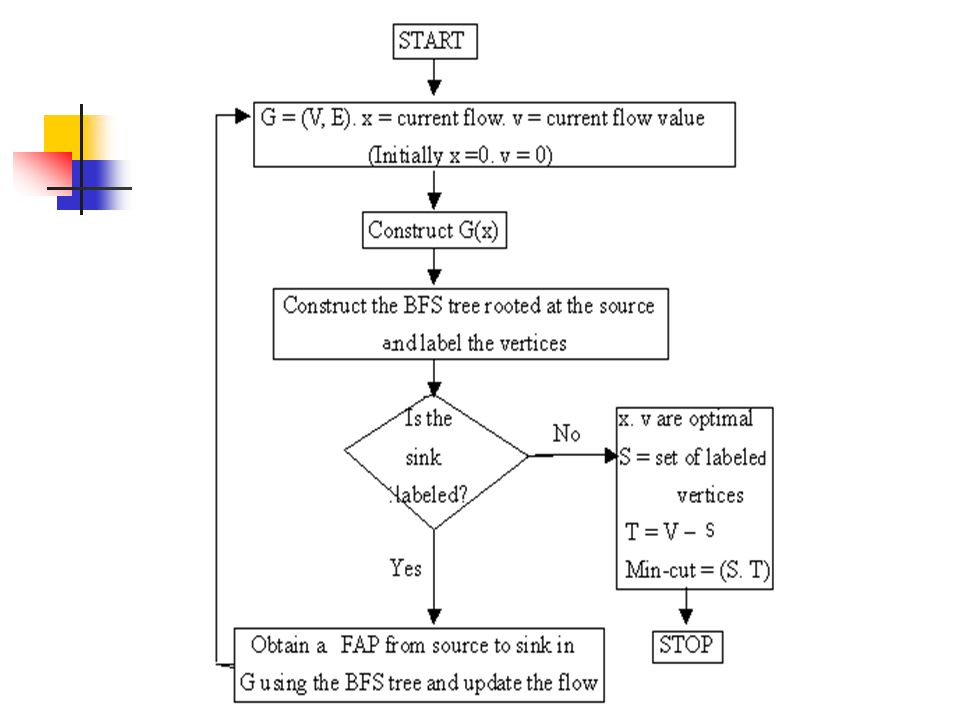
According to the flow chart, each iteration consists of 5 steps: Step1. Use the current flow x to display G, with each arc showing both the flow and the capacity. Step 2. Construct the residual network G(x). Step 3. Construct the BFS tree rooted at the source in G(x) with labeled and unlabeled vertices. Stop if the sink cannot be labeled, in which case x is optimal. Otherwise go to step 4. Step 4. Construct an FAP. Step 5. Update the flow and go to step 1.

Example 4.6: Find the maximum flow from vertex 1 to 6 in the given network by the labeling algorithm.

Iteration 1: (start with x = 0) Step 1: Show x & u (v=0) Step 2: Construct G(x)

Step 2: Step 3: Construct BFS tree

Step 3: The sink is labeled. Step 4: Find FAP

Step 5: Update the flow Flow is updated and

Iteration 2: Step 1: Show x & u (v = 4) Step 2: Construxt G(x)

Step 2: Step 3: Find BFS tree

Step 3: Step 4: Find FAP The sink is labeled.

Step 4: The sink is labeled. Step 5: Update the flow The flow is updated and

Iteration 3: Step 1: Show x & u (v = 5) Step 2: Give G(x)

Step 2: Step 3: Find BFS tree

Step 3: Step 4: Find FAP The sink is labeled.

Step 4: The sink is labeled. Step 5: Update the flow Flow is updated and

Iteration 4: Step 1: Show x & u (v = 7) Step 2: Give G(x)

Step 2: Step 3: BFS tree

Step 4: The sink has no label. No FAP. Current flow in Step 1 is optimal. S = {1, 3} and T = {2, 4, 5, 6}. Min-cut is (S, T) ={(1, 2), (3, 4)}. Min-cut value = max-flow value = 7.

Use NETSOLVE to calculate Min-Cost Flow Problem
Specify that it is a directed network. Need to enter node data: node name and supply. For the supply entry, type positive value if it is a source; negative value if it is a sink; and 0 if it is an intermediate. Need to enter arc data. For each arc, enter the starting node name, the ending node name, the cost, the lower bound of flow (usually 0), and the upper bound (i.e. the capacity) of the arc by this order. The command to solve such problems is MINFLOW.

Use NETSOLVE to calculate Min-Cost Flow Problem
For Example 4.1, for node data, type (6 lines): 1 9 2 -4 …… 6 8 and for edge data, type (11 lines):

Use NETSOLVE to calculate Maximum Flow Problem
Specify that it is a directed network. Do not need to enter node data. Need to enter arc data: for each arc, type the starting node name, the ending node name, 1 (as the cost even though this parameter is not used), 0 (the lower bound of flow), and the capacity by this order. If you want to find the maximum flow, say, from node 1 to node 9, type command: maxflow 1 9

Use NETSOLVE to calculate Maximum Flow Problem
For Example 4.6, the arc data should be typed as (7 lines): ……

Chapter 4 Minimum Cost Flow Problems (MCF)

Similar presentations

Presentation on theme: "Chapter 4 Minimum Cost Flow Problems (MCF)"— Presentation transcript:

Similar presentations

About project

Feedback

Log in

Auth with social network:

Chapter 4 Minimum Cost Flow Problems (MCF)

Similar presentations

Presentation on theme: "Chapter 4 Minimum Cost Flow Problems (MCF)"— Presentation transcript:

Similar presentations

About project

Feedback