Download presentation
Presentation is loading. Please wait.

10
Introduction --Classification Shape ContourRegion Structural Syntactic Graph Tree Model-driven Data-driven Perimeter Compactness Eccentricity Fourier Descriptors Wavelet Descriptors Curvature Scale Space Shape Signature Chain Code Hausdorff Distance Elastic Matching Non-Structural Area Euler Number Eccentricity Geometric Moments Zernike Moments Pseudo-Zernike Mmts Legendre Moments Grid Method

11
Boundary Descriptors There are several simple geometric measures that can be useful for describing a boundary. There are several simple geometric measures that can be useful for describing a boundary. –The length of a boundary: the number of pixels along a boundary gives a rough approximation of its length. –Curvature: the rate of change of slope To measure a curvature accurately at a point in a digital boundary is difficult To measure a curvature accurately at a point in a digital boundary is difficult The difference between the slops of adjacent boundary segments is used as a descriptor of curvature at the point of intersection of segments The difference between the slops of adjacent boundary segments is used as a descriptor of curvature at the point of intersection of segments

12
Volumetric Representations Represent models by the volume that they occupy: Represent models by the volume that they occupy: Rasterize the models into a binary voxel grid Rasterize the models into a binary voxel grid –A voxel has value 1 if it is inside the model –A voxel has value 0 if it is outside Model Voxel Grid

13
Shape Descriptors Representation: Representation: –What can you represent? –What are you representing? Matching: Matching: –How do you align? –Part or whole matching? Point Clouds Polygon SoupsClosed MeshesGenus-0 Meshes Shape Spectrum

14
Light Field Descriptor Hybrid boundary/volume representation Hybrid boundary/volume representation Model Image BoundaryVolume [Chen et al. 2003]

17
Representation Chain Codes Representation Chain Codes

18
Boundary Descriptors Shape Numbers Boundary Descriptors Shape Numbers

19
Representation Polygonal Approximations Representation Polygonal Approximations Polygonal approximations: to represent a boundary by straight line segments, and a closed path becomes a polygon. Polygonal approximations: to represent a boundary by straight line segments, and a closed path becomes a polygon. The number of straight line segments used determines the accuracy of the approximation. The number of straight line segments used determines the accuracy of the approximation. Only the minimum required number of sides necessary to preserve the needed shape information should be used (Minimum perimeter polygons). Only the minimum required number of sides necessary to preserve the needed shape information should be used (Minimum perimeter polygons). A larger number of sides will only add noise to the model. A larger number of sides will only add noise to the model.
. Only the minimum required number of sides necessary to preserve the needed shape information should be used (Minimum perimeter polygons). A larger number of sides will only add noise to the model. A larger number of sides will only add noise to the model..")
23
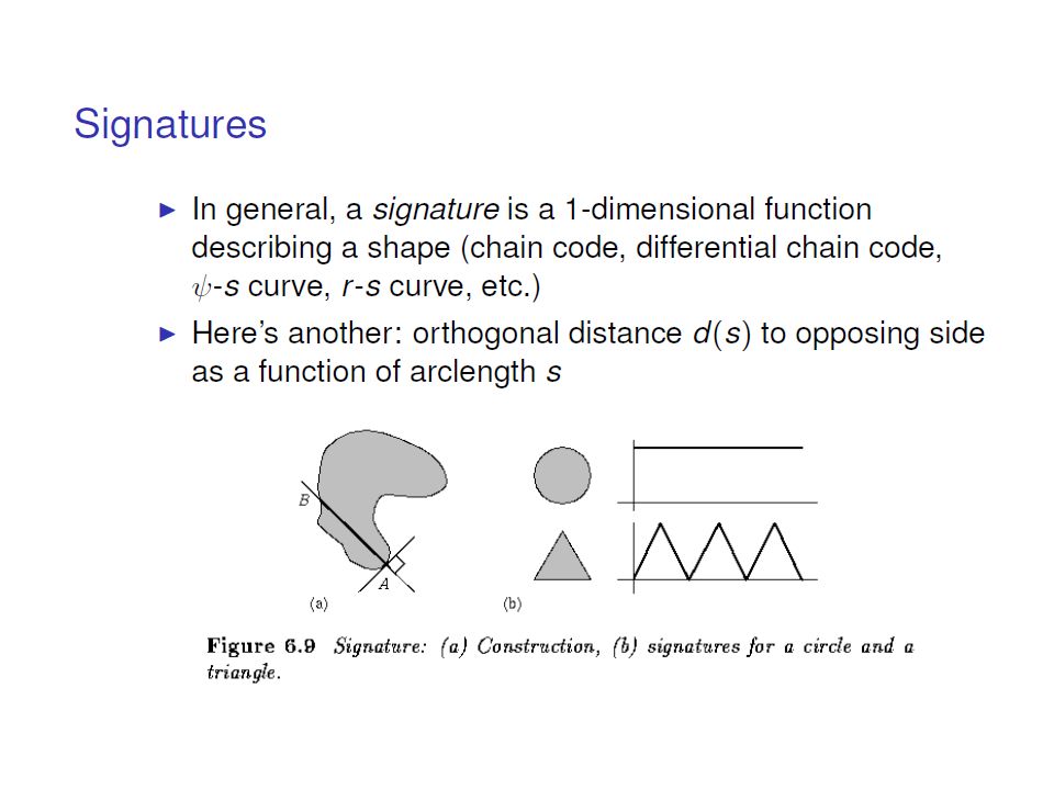
Signatures are invariant to location, but will depend on rotation and scaling. Signatures are invariant to location, but will depend on rotation and scaling. –Starting at the point farthest from the reference point or using the major axis of the region can be used to decrease dependence on rotation. –Scale invariance can be achieved by either scaling the signature function to fixed amplitude or by dividing the function values by the standard deviation of the function. Representation Signature Representation Signature

28
Representation Polygonal Approximations Representation Polygonal Approximations Minimum perimeter polygons: (Merging and splitting) Minimum perimeter polygons: (Merging and splitting) –Merging and splitting are often used together to ensure that vertices appear where they would naturally in the boundary. –A least squares criterion to a straight line is used to stop the processing.

45
Representation Skeletons Representation Skeletons Skeletons: produce a one pixel wide graph that has the same basic shape of the region, like a stick figure of a human. It can be used to analyze the geometric structure of a region which has bumps and “arms”. Skeletons: produce a one pixel wide graph that has the same basic shape of the region, like a stick figure of a human. It can be used to analyze the geometric structure of a region which has bumps and “arms”.

46
One application of skeletonization is for character recognition. One application of skeletonization is for character recognition. A letter or character is determined by the center-line of its strokes, and is unrelated to the width of the stroke lines. A letter or character is determined by the center-line of its strokes, and is unrelated to the width of the stroke lines. Representation Skeletons: Example Representation Skeletons: Example

47
Regional Descriptors Topological Descriptors Regional Descriptors Topological Descriptors Topological property 1: the number of holes (H) Topological property 2: the number of connected components (C)
 Topological property 2: the number of connected components (C)")
48
Regional Descriptors Topological Descriptors Regional Descriptors Topological Descriptors Topological property 3: Euler number: the number of connected components subtract the number of holes E = C - H E=0 E= -1

49
Regional Descriptors Topological Descriptors Regional Descriptors Topological Descriptors Topological property 4: the largest connected component.

50
Regional Descriptors Texture Regional Descriptors Texture

51
Regional Descriptors Texture Regional Descriptors Texture Texture is usually defined as the smoothness or roughness of a surface. Texture is usually defined as the smoothness or roughness of a surface. In computer vision, it is the visual appearance of the uniformity or lack of uniformity of brightness and color. In computer vision, it is the visual appearance of the uniformity or lack of uniformity of brightness and color. There are two types of texture: random and regular. There are two types of texture: random and regular. –Random texture cannot be exactly described by words or equations; it must be described statistically. The surface of a pile of dirt or rocks of many sizes would be random. –Regular texture can be described by words or equations or repeating pattern primitives. Clothes are frequently made with regularly repeating patterns. –Random texture is analyzed by statistical methods. –Regular texture is analyzed by structural or spectral (Fourier) methods.
 methods..")
52
Regional Descriptors Statistical Approaches Regional Descriptors Statistical Approaches Let z be a random variable denoting gray levels and let p(z i ), i=0,1,…,L-1, be the corresponding histogram, where L is the number of distinct gray levels. Let z be a random variable denoting gray levels and let p(z i ), i=0,1,…,L-1, be the corresponding histogram, where L is the number of distinct gray levels. –The nth moment of z: –The measure R: –The uniformity: –The average entropy:
, i=0,1,…,L-1, be the corresponding histogram, where L is the number of distinct gray levels. –The nth moment of z: –The measure R: –The uniformity: –The average entropy:.")
53
Regional Descriptors Statistical Approaches Regional Descriptors Statistical Approaches Smooth Coarse Regular

55
Regional Descriptors Spectral Approaches Regional Descriptors Spectral Approaches

56
Regional Descriptors Spectral Approaches Regional Descriptors Spectral Approaches

57
Regional Descriptors Moments of Two-Dimensional Functions Regional Descriptors Moments of Two-Dimensional Functions For a 2-D continuous function f(x,y), the moment of order (p+q) is defined as For a 2-D continuous function f(x,y), the moment of order (p+q) is defined as The central moments are defined as The central moments are defined as
, the moment of order (p+q) is defined as For a 2-D continuous function f(x,y), the moment of order (p+q) is defined as The central moments are defined as The central moments are defined as")
58
Regional Descriptors Moments of Two-Dimensional Functions Regional Descriptors Moments of Two-Dimensional Functions If f(x,y) is a digital image, then If f(x,y) is a digital image, then The central moments of order up to 3 are The central moments of order up to 3 are
 is a digital image, then If f(x,y) is a digital image, then The central moments of order up to 3 are The central moments of order up to 3 are")
59
Regional Descriptors Moments of Two-Dimensional Functions Regional Descriptors Moments of Two-Dimensional Functions The central moments of order up to 3 are The central moments of order up to 3 are

60
Regional Descriptors Moments of Two-Dimensional Functions Regional Descriptors Moments of Two-Dimensional Functions The normalized central moments are defined as The normalized central moments are defined as

61
Regional Descriptors Moments of Two-Dimensional Functions Regional Descriptors Moments of Two-Dimensional Functions A seven invariant moments can be derived from the second and third moments: A seven invariant moments can be derived from the second and third moments:

62
Regional Descriptors Moments of Two-Dimensional Functions Regional Descriptors Moments of Two-Dimensional Functions This set of moments is invariant to translation, rotation, and scale change. This set of moments is invariant to translation, rotation, and scale change.

63
Regional Descriptors Moments of Two-Dimensional Functions Regional Descriptors Moments of Two-Dimensional Functions

64
Table 11.3 Moment invariants for the images in Figs. 11.25(a)-(e). Regional Descriptors Moments of Two-Dimensional Functions Regional Descriptors Moments of Two-Dimensional Functions
-(e). Regional Descriptors Moments of Two-Dimensional Functions Regional Descriptors Moments of Two-Dimensional Functions.")
67
The End

Similar presentations


>")


 Dr.Çağatay ÜNDEĞER Instructor Middle East Technical University, GameTechnologies & General Manager SimBT.>")


>")