1. Copyright © 2009 by The McGraw-Hill Companies, Inc. All rights reserved. McGraw-Hill/Irwin Lecture 3 [Chapter 3]

2.  Demand and its determinants  Supply and its determinants  Supply, demand, & market equilibrium  Changes in supply and demand  Government-set prices 3-2

3.  Interaction between buyers and sellers  Buyers demand goods  Sellers supply goods  Assumptions  Standardized good  Competitive market 3-3

4.  Schedule or curve  Amount consumers willing and able to purchase at a given price  Other things equal  Individual demand  Market demand 3-4

5.  Other things equal, as price falls quantity demanded rises  Explanations:  Diminishing marginal utility  Income effect  Substitution effect 3-5

6. 6 5 4 3 2 1 0 10 20 30 40 50 60 70 80 Quantity Demanded (bushels per week) Price (per bushel) PQdQd $5 4 3 2 1 10 20 35 55 80 P Q D 3-6

7.  Common sense among consumers  Diminishing Marginal utility  Income and Substitution effects

8. The quantities demanded by all consumers at each price are added.

9.  Summing the plotted graphs of individual demand schedules and combining them into one illustration yields the market demand.

10. 6 5 4 3 2 1 0 Quantity Demanded (bushels per week) Price (per bushel) PQdQd $5 4 3 2 1 10 20 35 55 80 Individual Demand P Q D1D1 2 4 6 8 10 12 14 16 18 Demand Can Increase or Decrease Decrease in Demand D2D2 D3D3 Change in Demand Change in Quantity Demanded 3-10

11.  A change in the price of a product causes a change in quantity demanded, and is represented by a movement along a downward-sloping demand curve from one point to another point.  Other factors can and do affect purchases. If any of these factors change, the demand curve will shift to the right or left. These factors, called determinants of demand, are sometimes referred to as demand shifters. A shift in the demand curve is called a change in demand.

12.  Factors that shift the demand curve to the right or left include changes in:  Consumer tastes (or preferences)  Number of buyers  Income  Normal goods – products whose demand varies directly with money income.  Inferior goods - products whose demand varies inversely with money income. 3-12

13.  Price of related goods  Substitute good  Complementary good  Unrelated goods  Consumer expectations about future prices or incomes 3-13

14.  The way in which goods relate to other goods may impact demand as well.  A substitute good is one that can be used in place of another good.  A complementary good is one that is used together with another good.  Unrelated goods are not related in consumption.

15.  Supply: the quantities of a product that producers are willing and able to make available for sale at various possible prices.  The Law of Supply: a positive or direct relationship between price and quantity supplied exists, other things equal.  Supply is upward sloping:  As price rises (falls), the quantity supplied rises (falls). 3-15

16.  Explanations:  Revenue implications  Marginal cost 3-16

17. 6 5 4 3 2 1 0 Quantity Supplied (bushels per week) Price (per bushel) PQsQs $5 4 3 2 1 60 50 35 20 5 Individual Supply P Q S1S1 10 20 30 40 50 60 70 3-17

18. 6 5 4 3 2 1 0 Quantity Supplied (bushels per week) Price (per bushel) PQsQs $5 4 3 2 1 60 50 35 20 5 Individual Supply P Q S1S1 Supply Can Increase or Decrease S2S2 S3S3 10 20 30 40 50 60 70 3-18

19. 6 5 4 3 2 1 0 Quantity Supplied (bushels per week) Price (per bushel) PQsQs $5 4 3 2 1 60 50 35 20 5 Individual Supply P Q S1S1 Supply Can Increase or Decrease S2S2 S3S3 10 20 30 40 50 60 70 Change in Quantity Supplied Change in Supply 3-19

20.  Resource prices  Technology  Taxes and subsidies  Prices of other goods  Producer expectations  Number of sellers 3-20

21.  The point at which the market demand curve and market supply curves intersect  Equilibrium Price is the market clearing price.  Qty demanded and qty supplied are equal at the equilibrium price.  NO Surplus and NO shortage 3-21

22. 6 5 4 3 2 1 0 2 4 6 8 10 12 14 16 18 Bushels of Corn (thousands per week) Price (per bushel) PQdQd $5 4 3 2 1 2,000 4,000 7,000 11,000 16,000 Market Demand 200 Buyers PQsQs $5 4 3 2 1 12,000 10,000 7,000 4,000 1,000 Market Supply 200 Sellers 200 Buyers & 200 Sellers 7 3 D S $4 Price Floor 6,000 Bushel Surplus $2 Price Ceiling 7,000 Bushel Shortage 3-22

23.  The Rationing function of prices is the ability of the competitive forces of supply and demand to establish a price at which selling and buying decisions are consistent  Efficient allocation  Productive efficiency : The production of any particular good or service in the least costly way  Allocative efficiency: The particular mix of goods and services most highly valued by society

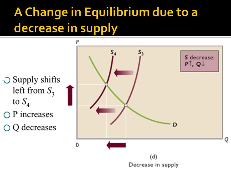
24.  A shift in either a demand curve or supply curve represents a change in equilibrium  Constant supply, demand increases – equilibrium P & Q rise  Constant supply, demand decreases – equilibrium P & Q fall  Constant demand, supply increases – equilibrium P falls & equilibrium Q rises  Constant demand, supply decreases – equilibrium P rises & equilibrium Q falls 3-24

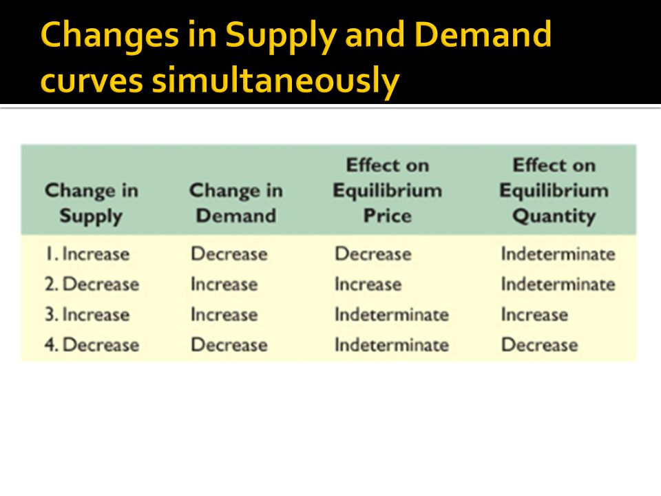
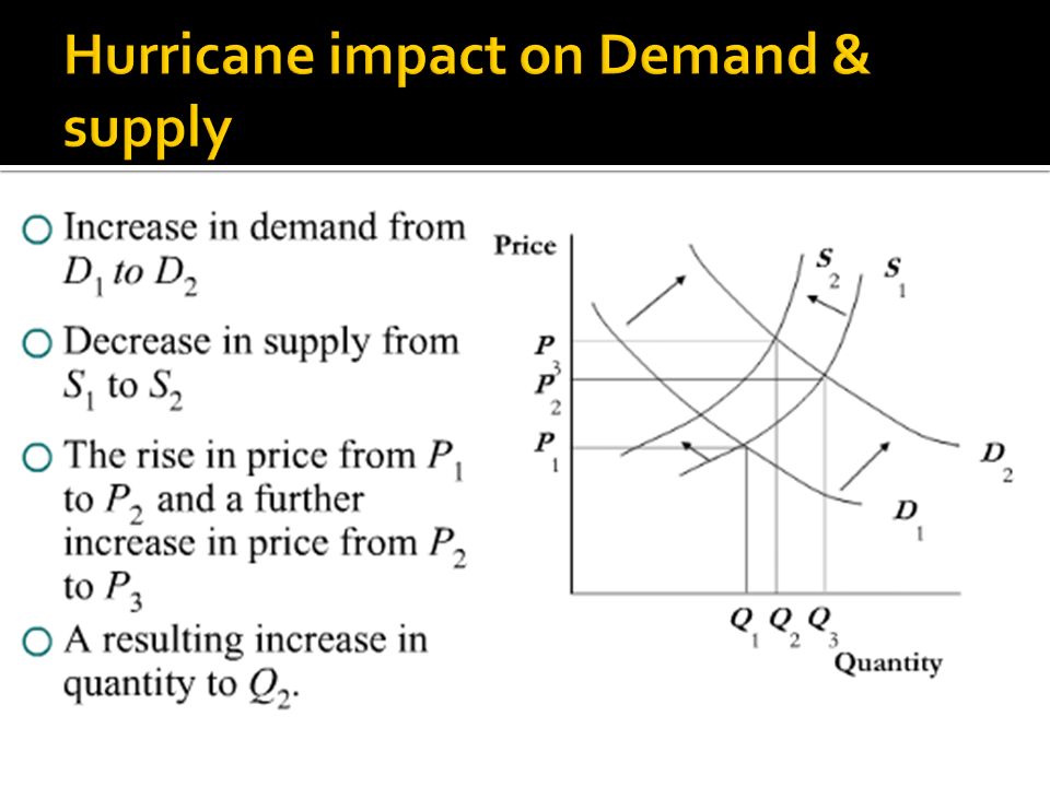
26.  When both Supply and Demand change, the effect is a combination of the individual effects.  These complex cases include:  Increase in Supply; decrease in Demand  Decrease in Supply; increase in Demand  Increase in Supply; increase in Demand  Decrease in Supply; decrease in Demand 3-26

29.  Equilibrium prices deemed unfairly high for buyers or unfairly low for sellers.  Government controlled prices in the form of ceilings and floors.  Results in market disequilibrium, blocks the rationing function of prices and distorts resource allocations.

30.  One interference with the market process is called a Price Ceiling  A price ceiling occurs when the price is artificially held below the equilibrium price and is not allowed to rise.  Involve the government in some way  Examples: Rent control, gasoline prices,  Price ceilings lead to shortages.  Shortages create a rationing problem

31.  Equilibriu m price is $3.50  Price Ceiling set at $3.00  Shortage: (Q s – Q d ) is negative 3-31

32.  Price ceilings provide a gain for buyers and a loss for sellers.  Sellers would like to avoid the loss if they can. 1. Black market: In this case, the sellers illegally raise the price and hope to get away with it. So, for example, tickets to popular events are sold by scalpers at high prices.  While there are many other examples, black markets are not smart; it is just too easy to be caught. It is also not smart because of the existence of gray markets. 2. A gray market is a way of getting around the price ceiling without actually doing anything illegal. There are two forms of gray market.  One form of gray market involves charging for goods or services that were formerly provided free  The second form of gray market is to provide less service for the same price

33.  A price floor exists when the price is artificially held above the equilibrium price and is not allowed to fall.  Price floors always generate surpluses.

34.  Equilibrium price is $2  Price floor set at $3  Surplus: (Q s – Q d ) is positive

35.  Keep more producers in business  Fail to achieve allocative effeciency  Increase in tax burden created by subsidy payments to producers  Consumers gain nothing and ultimately pay high prices

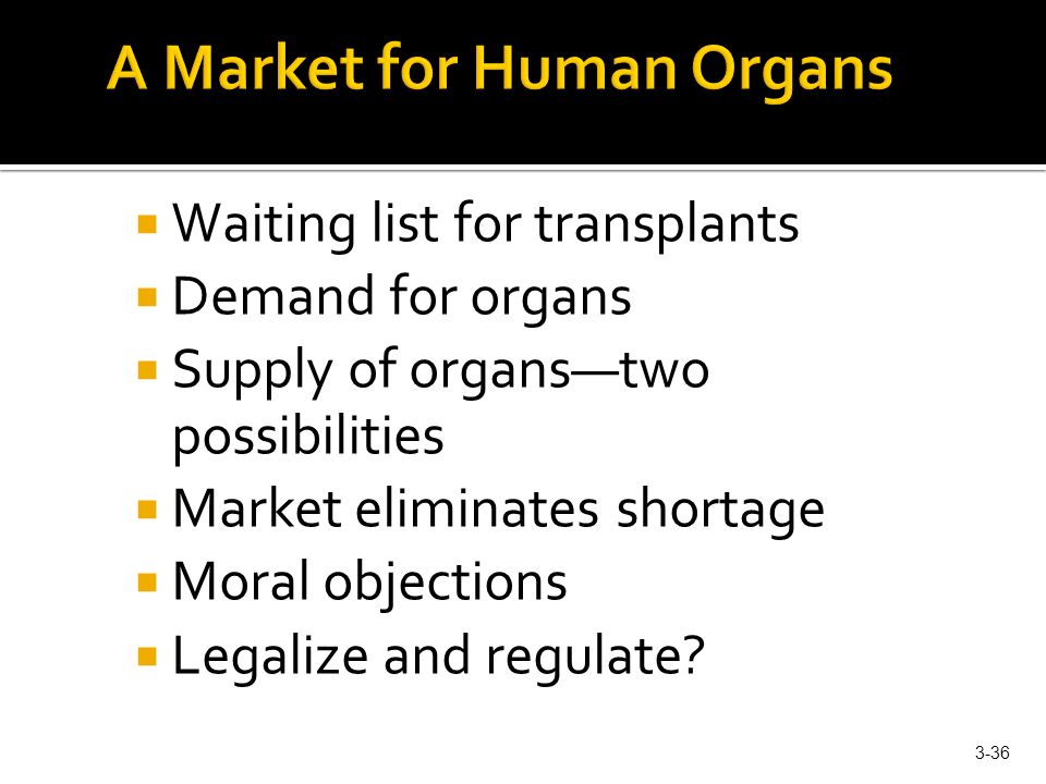
36.  Waiting list for transplants  Demand for organs  Supply of organs—two possibilities  Market eliminates shortage  Moral objections  Legalize and regulate? 3-36

37. P Q S2S2 S1S1 D1D1 P1P1 P0P0 Q1Q1 Q2Q2 Q3Q3 Supply of Organs Shortage at Zero Price Q 1 – Q 3 At Price P 1 the Shortage is Reduced By Q 1 – Q 2 Demand for Organs 3-37

38.  demand  demand schedule  law of demand  diminishing marginal utility  income effect  substitution effect  demand curve  determinants of demand  normal goods  inferior goods  substitute good  complementary good  change in demand  change in quantity demanded  supply  supply schedule  law of supply  supply curve  determinants of supply  change in supply  change in quantity supplied  equilibrium price  equilibrium quantity  surplus  shortage  price ceiling  price floor 3-38

39. Elasticity, Consumer Surplus, and Producer Surplus 3-39