1. Ch. 5 Linear Models & Matrix Algebra
5.1 Conditions for Nonsingularity of a Matrix 5.2 Test of Nonsingularity by Use of Determinant
5.3 Basic Properties of Determinants
5.4 Finding the Inverse Matrix
5.5 Cramer's Rule
5.6 Application to Market and National-Income Models
5.7 Leontief Input-Output Models
5.8 Limitations of Static Analysis

2. x + y = 8 x + y = 9 (inconsistent & dependent)
5.1 Conditions for Nonsingularity of a Matrix 3.4 Solution of a General-equilibrium System (p. 44)
x + y = 8 x + y = 9 (inconsistent & dependent)
2x + y = 12 4x + 2y= 24 (dependent)
2x + 3y = 58 y = 18 x + y = 20 (over identified & dependent)

3. Sometimes one equation is a multiple of the other. (redundant)
5.1 Conditions for Non-singularity of a Matrix 3.4 Solution of a General-equilibrium System (p. 44) y x
x + y = 9
x + y = 8
Sometimes equations are not consistent, and they produce two parallel lines. (contradict)
Sometimes one equation is a multiple of the other. (redundant) y 12
For both the equations
Slope is -1

4. B) Rows (cols.) linearly independent (rank=n, sufficient)
5.1 Conditions for Non-singularity of a Matrix Necessary versus sufficient conditions Conditions for non-singularity Rank of a matrix
A) Square matrix , i.e., n. equations = n. unknowns. Then we may have unique solution. (nxn , necessary)
B) Rows (cols.) linearly independent (rank=n, sufficient)
A & B (nxn, rank=n) (necessary & sufficient), then nonsingular

5. 5.1 Elementary Row Operations (p. 86)
Interchange any two rows in a matrix
Multiply or divide any row by a scalar k (k  0)
Addition of k times any row to another row
These operations will:
transform a matrix into a reduced echelon matrix (or identity matrix if possible)
not alter the rank of the matrix
place all non-zero rows before the zero rows in which non-zero rows reveal the rank

6. 5.1 Conditions for Nonsingularity of a Matrix Conditions for non-singularity, Rank of a matrix (p. 86)

7. 5.1 Conditions for Non-singularity of a Matrix Conditions for non-singularity, Rank of a matrix (p. 96)

8. 5.1 Conditions for Nonsingularity of a Matrix Conditions for non-singularity, Rank of a matrix (p. 96)

9. 5.1 Conditions for Non-singularity of a Matrix Conditions for non-singularity, Rank of a matrix (p. 96)

10. 5.2 Test of Non-singularity by Use of Determinant Determinants and non-singularity Evaluating a third-order determinant Evaluating an nth order determent by Laplace expansion
Determinant |A| is a uniquely defined scalar associated w/ a square matrix A (Chiang & Wainwright, p. 88)
|A| defined as the sum of all possible products t(-1)t a1j a2k…ang, where the series of second subscripts is a permutation of (1,.., n) including the natural order (1, …, n), and t is the number of transpositions required to change a permutation back into the original order (Roberts & Schultz, p )
t equals P(n,r)=n!/(n-r)!, i.e., the permutation of n objects taken r at a time

11. 5.2 Test of Non-singularity by Use of Determinant
P(n,r) = n!/(n-r)! P(2,2) = 2!/(2-2)! = 2
There are only two ways of arranging subscripts (i,k) of product (-1)ta1ja2k either (1,2) or (2,1)
The first permutation is even & positive (-1)2 and second is odd and negative (-1)1
0!=(1) = 1 1!=(1) = 1 2!=(2)(1) = 2 3!=(3)(2)(1) = 6 4!=(4)(3)(2)(1) = 24 5!=(5)(4)(3)(2)(1) = !=(6)(4)(3)(2)(1) = 720 … … 10! =3,628,800

12. 5.2 Test of Non-singularity by Use of Determinant and permutations: 2x2 and 3x3

13. 5.2 Test of Non-singularity by Use of Determinant : 4 x 4 permutations = 24
Abcd
Bacd
Cabd
Dabc
Abdc
Badc
Cadb
Dacb
Acbd
Bcad
Cbad
Dbac
Acdb
Bcda
Cbda
Dbca
Adbc
Bdac
Cdab
Dcab
Adcb
Bdca
Cdba
Dcba

14. 5.2 Evaluating a third-order determinant Evaluating an 3 order determent by Laplace expansion
Laplace Expansion by cofactors; if /A/ = 0, then /A/ is singular, i.e., under identified

15. 5.2 Determinants
Pattern of the signs for cofactor minors

16. 5.1 Conditions for Nonsingularity of a Matrix Conditions for non-singularity, Rank of a matrix (p. 96)

17. 5.1 Conditions for Non-singularity of a Matrix Conditions for non-singularity, Rank of a matrix (p. 96)

18. 5.2 Evaluating a determinant
Laplace expansion of a 3rd order determinant by cofactors. If /A/ = 0, then singular

19. 5.2 Test of Non-singularity by Use of Determinant
P(3,3) = 3!/(3-3)! = 6
|A| = 1(5)9 + 2(6)7 + 3(8)4 -3(5)7 – 6(8)1 – 9(4)2
Expansion by cofactors |A|= (1)c11 + (2)c12 + (3)c13
C11 = 5(9) – 6(8)
C12 = -4(9) + 6(7)
C13 = 4(8) – 7(5)
Expansion across any row or column will give the same # for the determinant

20. 5.3 Basic Properties of Determinants Properties I to III (related to elementary row operations)
The interchange of any two rows will alter the sign but not its numerical value
The multiplication of any one row by a scalar k will change its value k-fold
The addition of a multiple of any row to another row will leave it unaltered.

21. 5.3 Basic Properties of Determinants Properties IV to VI
The interchange of rows and columns does not affect its value
If one row is a multiple of another row, the determinant is zero
The expansion of a determinant by alien cofactors produces a result of zero

22. 5.3 Basic Properties of Determinants Properties I to V
If /A/  0
Then
A is nonsingular
A-1 exists
A unique solution to
X=A-1d exists
/A/ = /A'/
Changing rows or col. does not change # but changes the sign of /A/
k(row) = k/A/
ka ± row or col.b =/A/
If row or col a=kb, then /A/ =0

23. 5.4 Finding the Inverse aka “the hard way”
Steps in computing the Inverse Matrix and solving for x
1.  Find the determinant |A| using expansion by cofactors.
If |A| =0, the inverse does not exist.
2.  Use cofactors from step 1 and complete the cofactor matrix.
3.   Transpose the cofactor matrix => adjA 
4. Divide adj.A by |A| => A-1
5. Post multiply matrix A-1 by column vector of constants d to solve for the vector of variables x

24. A= C=
C’=

25. 5.4 Finding the Inverse Matrix Expansion of a determinant by alien cofactors, Property VI, Matrix inversion
Expansion by alien cofactors yields /A/=0
This property of determinants is important when defining the inverse (A-1)

26. 5.4 A Inverse (A-1) Inverse of A is A-1
if and only if A is square (nxn) and rank = n
AA-1 = A-1A = I
We are interested in A-1 because x=A-1d

27. 5.4 matrix A: matrix of parameters from the equation Ax=d

28. C: Matrix of cofactors of A

29. C' or adjoint A: Transpose matrix of the cofactors of A

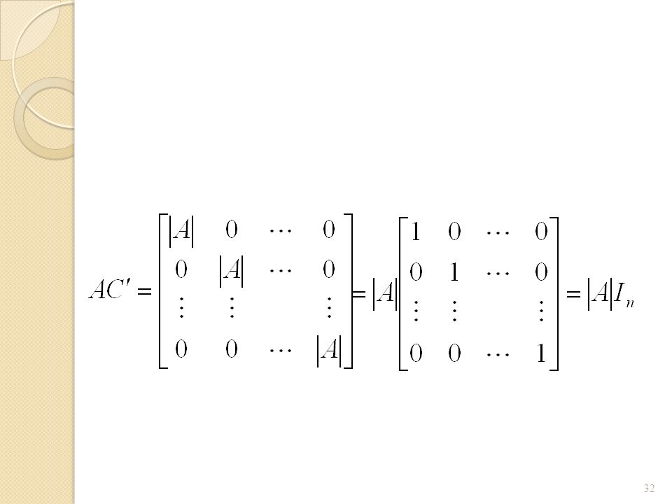
30. AC'

31. Matrix AC'

33. Inverse of A

34. Solving for X using Matrix Inversion

35. 5.4 A Inverse, solving for P

36. Cramer’s rule

37. Cramer's rule

38. Cramer's rule

39. Deriving Cramer’s Rule

40. 5.4 Finding the Inverse aka “the hard way”
Steps in computing the Inverse Matrix and solving for x
1.  Find the determinant |A| using expansion by cofactors.
If |A| =0, the inverse does not exist.
2.  Use cofactors from step 1 and complete the cofactor matrix.
3.   Transpose the cofactor matrix => adjA 
4. Divide adj.A by |A| => A-1
5. Post multiply matrix A-1 by column vector of constants d to solve for the vector of variables x

41. Derivation of matrix inverse formula
|A| = ai1ci1 + …. + aincin (scalar)
Adj. A = transposed cofactor matrix of A
A(adj.A)=|A|I (expansion by alien cofactors = 0 for off diagonal elements)
A(adj.A)/|A| = I
A-1 = (adj.A)/|A| QED Roberts & Schultz, p. 97-8)

42. 5.4 Finding the Inverse aka “the hard way”
Steps in computing the Inverse Matrix and solving for x
1.  Find the determinant |A| using expansion by cofactors.
If |A| =0, the inverse does not exist.
2.  Use cofactors from step 1 and complete the cofactor matrix.
3.   Transpose the cofactor matrix => adjA 
4. Divide adj.A by |A| => A-1
5. Post multiply matrix A-1 by column vector of constants d to solve for the vector of variables x

43. 5.4 A Inverse A(adjA) = |A|I A(adjA)/|A| = I ( |A| is a scalar)
A-1A(adjA)/|A|= A- 1I
adjA/|A|= A-1

44. Finding the Determinant
Y = C+I0+G
C = a + b(Y-T0)
G = gY
1Y – 1C–1G = I0
-bY+1C+ 0G = a-bT0
-gY+0C+ 1G = 0

45. Derivation of matrix inverse formula
|A| = ai1ci1 + …. + aincin (scalar)
Adj. A = transposed cofactor matrix of A
A(adj.A)=|A|I (expansion by alien cofactors = 0 for off diagonal elements)
A(adj.A)/|A| = I
A-1 = (adj.A)/|A| QED Roberts & Schultz, p. 97-8)

46. 5.4 Finding the Inverse aka “the hard way”
Steps in computing the Inverse Matrix and solving for x
1.  Find the determinant |A| using expansion by cofactors.
If |A| =0, the inverse does not exist.
2.  Use cofactors from step 1 and complete the cofactor matrix.
3.   Transpose the cofactor matrix => adjA 
4. Divide adj.A by |A| => A-1
5. Post multiply matrix A-1 by column vector of constants d to solve for the vector of variables x

47. 5.4 A Inverse A(adjA) = |A|I A(adjA)/|A| = I ( |A| is a scalar)
A-1A(adjA)/|A|= A- 1I
adjA/|A|= A-1

48. 5.4 Inverse, an example

49. Finding the Determinant
Y = C+I0+G
C = a + b(Y-T0)
G = gY
1Y – 1C–1G = I0
-bY+1C+ 0G = a-bT0
-gY+0C+ 1G = 0

50. The macro model Y=C+I0+G 1Y - 1C – 1G = I0
C=a+b*(Y-T0) -bY + 1C + 0G = a-bT0
G=g*Y -gY + 0C +1G = 0 =

51. Macro model Section 3.5, Exercise 3.5-2 (a-d), p. 47
Section 5.6, Exercise (a-b), p. 111
Given the following model
(a) Identify the endogenous variables
(b) Give the economic meaning of the parameter g
(c) Find the equilibrium national income (substitution)
(d) What restriction on the parameters is needed for a solution to exist?
Find Y, C, G by (a) matrix inversion (b) Cramer’s rule

52. The macro model Y=C+I0+G 1Y - 1C – 1G = I0
C=a+b*(Y-T0) -bY + 1C + 0G = a-bT0
G=g*Y -gY + 0C +1G = 0 =

53. A= C=
C’=

54. 3.4 Solution of General Eq. System
(1)(1)-(1)(1) = 0 (inconsistent & dependent)
(2)(2)-(1)(4) = 0 (dependent)
(2)(1)-(1)(3) = -1 (independent as rewritten)

55. 5. 7 Leontief Input-Output Models. Structure of an input-output model
5.7 Leontief Input-Output Models Structure of an input-output model The open model, A numerical example Finding the inverse by approximation, The closed model
(I -A)x = d ; x = (I -A)-1 d

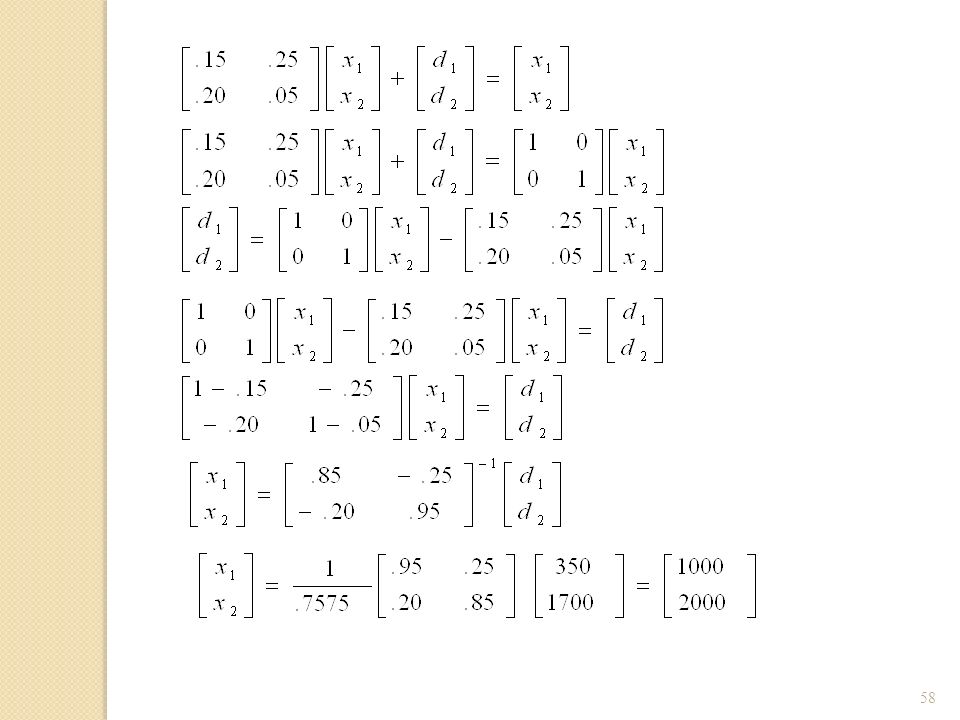
56. Sector 1 (a1jx1) Sector 2 (a2jx2) Final demand (di) Total output (xi)
Miller and Blair 2-3, Table 2-3, p 15 Economic Flows ($ millions) To
Sector 1 (a1jx1)
Sector 2 (a2jx2)
Final demand (di)
Total output (xi)
Sector 1
150
500
350
1000
Sector 2
200
100
1700
2000
Factor Payment (Wi)
650
1400
1100
3150
Total outlays (Xi)
6150
Sector 1 (aij)
Sector 2 (aij)
0.15
0.25
0.20
0.05
0.65
0.70
1.00

57. Leontief Input-output Analysis

59. 5.8 Limitations of Static Analysis
Static analysis solves for the endogenous variables for one equilibrium
Comparative statics show the shifts between equilibriums
Dynamics analysis looks at the attainability and stability of the equilibrium

60. 3.4 Solution of General Eq. System
(1)(1)-(1)(1) = 0 (inconsistent & dependent)
(2)(2)-(1)(4) = 0 (dependent)
(2)(1)-(1)(3) = -1 (independent as rewritten)

61. Why use matrix method at all? Compact notation
5.6 Application to Market and National-Income Models Market model National-income model Matrix algebra vs. elimination of variables
Why use matrix method at all?
Compact notation
Test existence of a unique solution
Handy solution expressions subject to manipulation