1. Simulation of spatially correlated discrete random variables Dan Dalthorp and Lisa Madsen Department of Statistics Oregon State University dalthorp@science.oregonstate.edu lmadsen@science.oregonstate.edu Outline I. Generating one pair of correlated discrete random variables. (a) Lognormal-Poisson hierarchy (b) Overlapping sums II. Generating a vector of correlated discrete random variables by overlapping sums III. Examples

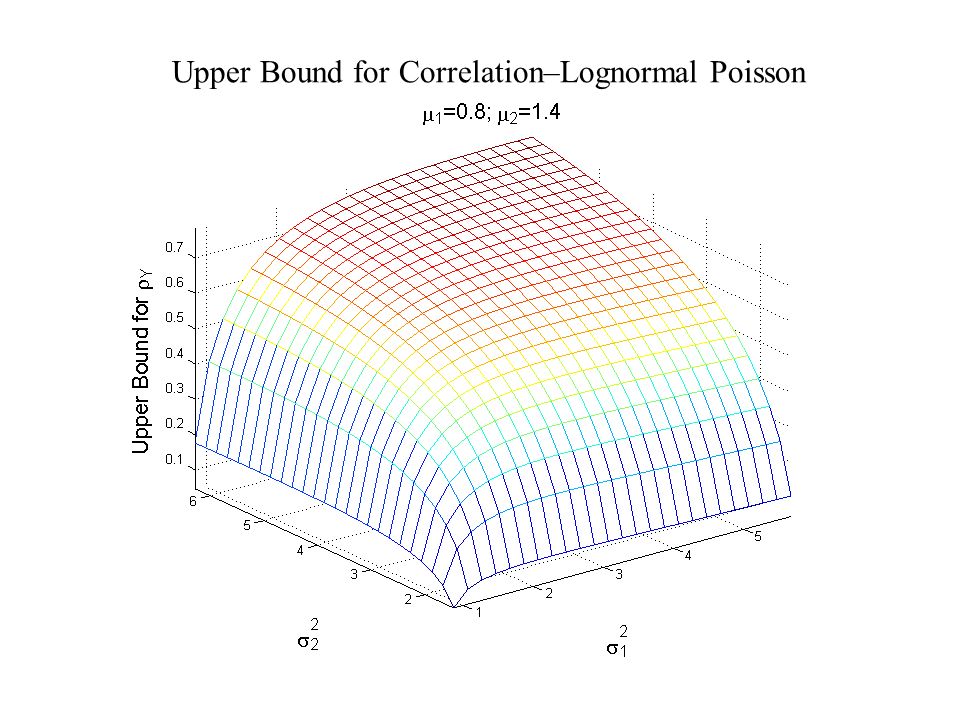
2. Introduction Generate Y 1, Y 2 where Y 1, Y 2 have specified means variances and correlation  Y  0 Y 1, Y 2 are count r.v.'s i.e., y = 0, 1, 2,... Distributions of Y 1, Y 2 are unimodal, Poisson-like If  2 < , then both  2 and  are small

3. Lognormal-Poisson Method For Generating Y 1 and Y 2 Generate correlated normal RVs Z 1, Z 2 Transform to lognormals X i = exp(Z i ) Y 1 and Y 2 resemble negative binomial RVs. Generate conditionally independent Y i ~ Poisson(X i )

4. Obtaining the Right Moments To get with corr(Y 1, Y 2 ) =  Y, generate lognormals X 1, X 2 with This requires normals Z 1, Z 2 with and

5. Constraints on Moments of Y 1, Y 2 with Lognormal-Poisson Method

6. Upper Bound for Correlation–Lognormal Poisson

8. Overlapping Sums Method For Generating Y 1 and Y 2 Generate independent, discrete RVs X 1, X 2, X Let Y 1 = X + X 1 Y 2 = X + X 2 Holgate (1964): Correlated Poissons We are not concerned with the exact distribution of Y 1 and Y 2, but we require them to be ecologically plausible.

9. Obtaining the Right Moments To get with corr(Y 1, Y 2 ) =  Y, Generate independent X 1, X 2, X with and

10. Choose distributions for Xs based on relationship between variance and mean: If, use X ~ Negative binomial(  X,  X 2 ) If, use X ~ Poisson(  X ) If, use X ~ Bernoulli(  X ) If and, use, where B~Bernoulli(p), and P~Poisson( ), with and then X cannot be simulated—by any method. If

11. Constraints on Moments of Y 1, Y 2 with Overlapping Sums Method No constraints on means of Y i, but we require ▪ Relationship between and ecologically plausible ▪

12. Upper Bound for Correlation–Overlapping Sums

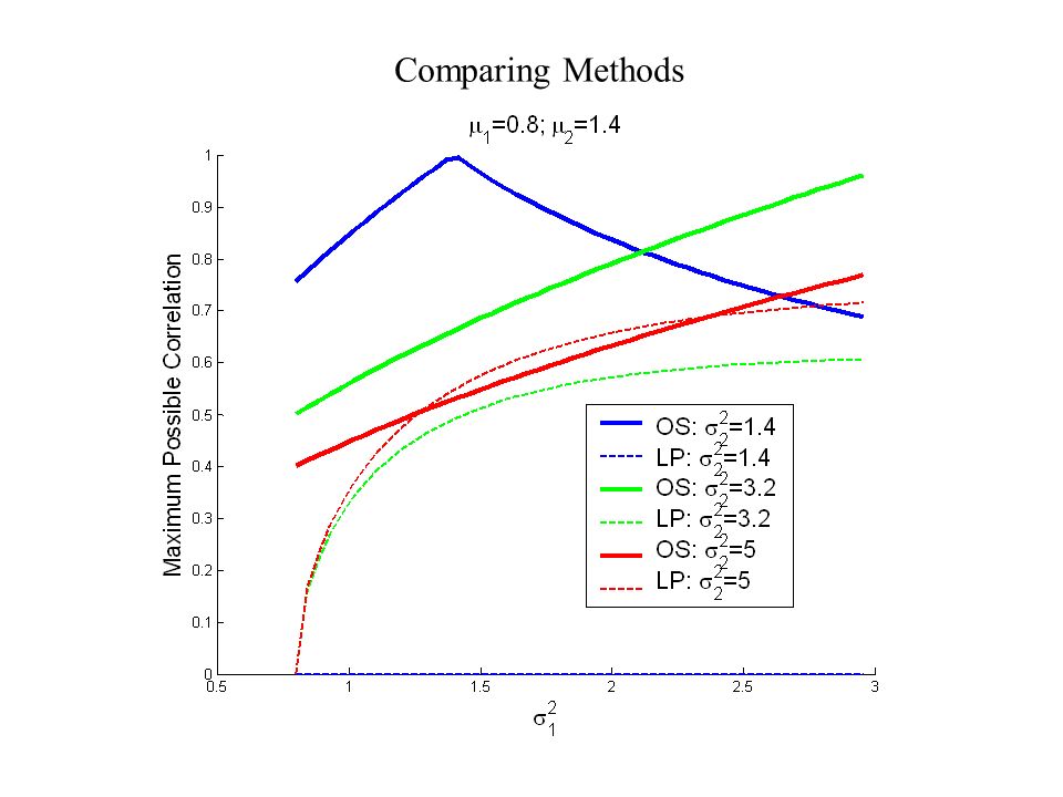
13. Comparing Methods

15. Step 1: Find variances and means of X's Y 1 = X + X 1 Y 2 = X + X 2 where X, X 1, and X 2 are independent count random variables with... Variances: Means: A quick example: Simulate Y 1 and Y 2 with and  = 0.2 Two equations, three unknowns... Try so X would be Bernoulli.

16. Step 2: Define distributions for X's X ~ Bernoulli(0.0921) since by design X 1 ~ Negative binomial with  = 0.928 and  2 = 1.172 X 2 = Bernoulli(p) + Poisson( ) with p = 0.05 and = 0.0079 Step 3: Simulate Y 1 = X + X 1 Y 2 = X + X 2

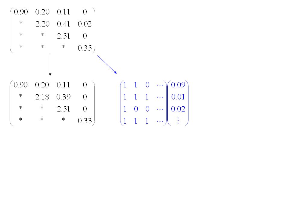
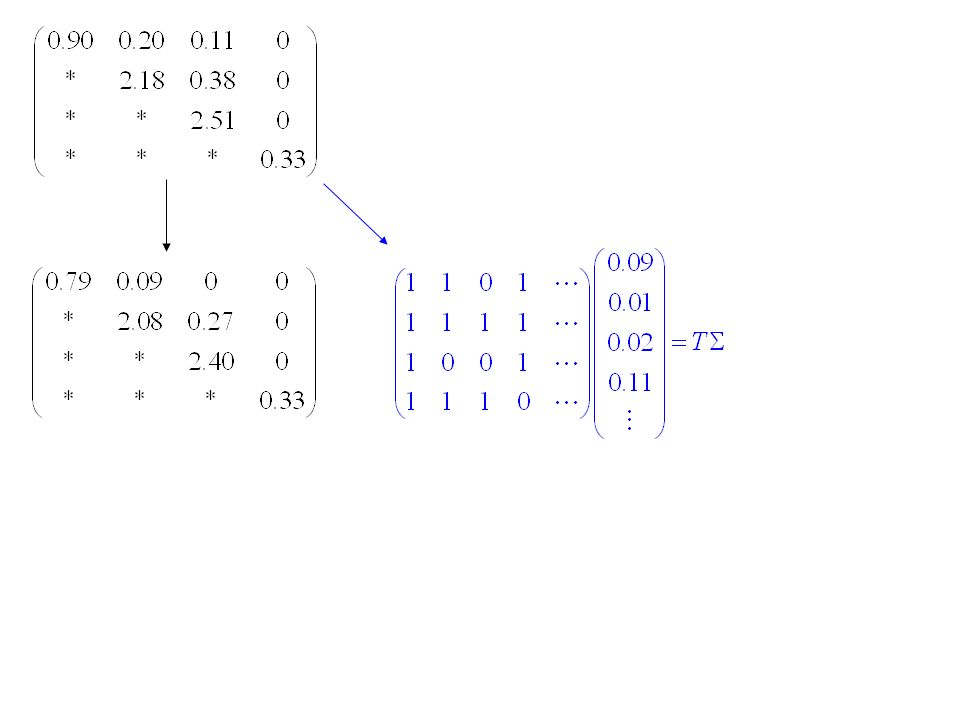
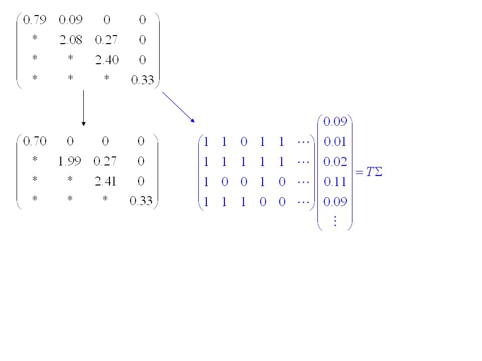
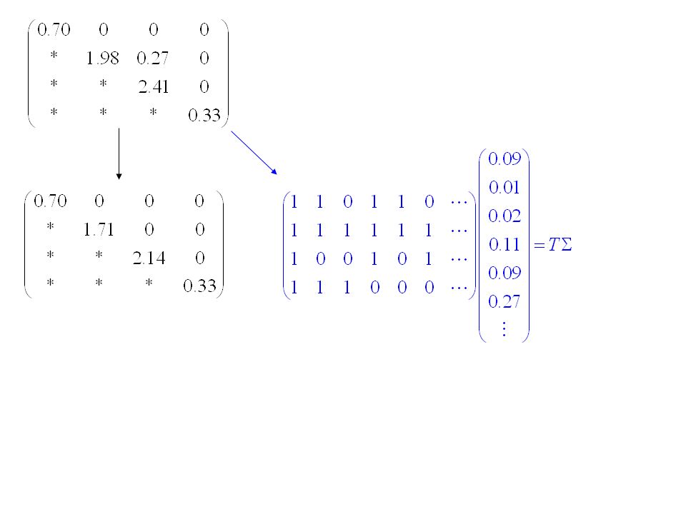
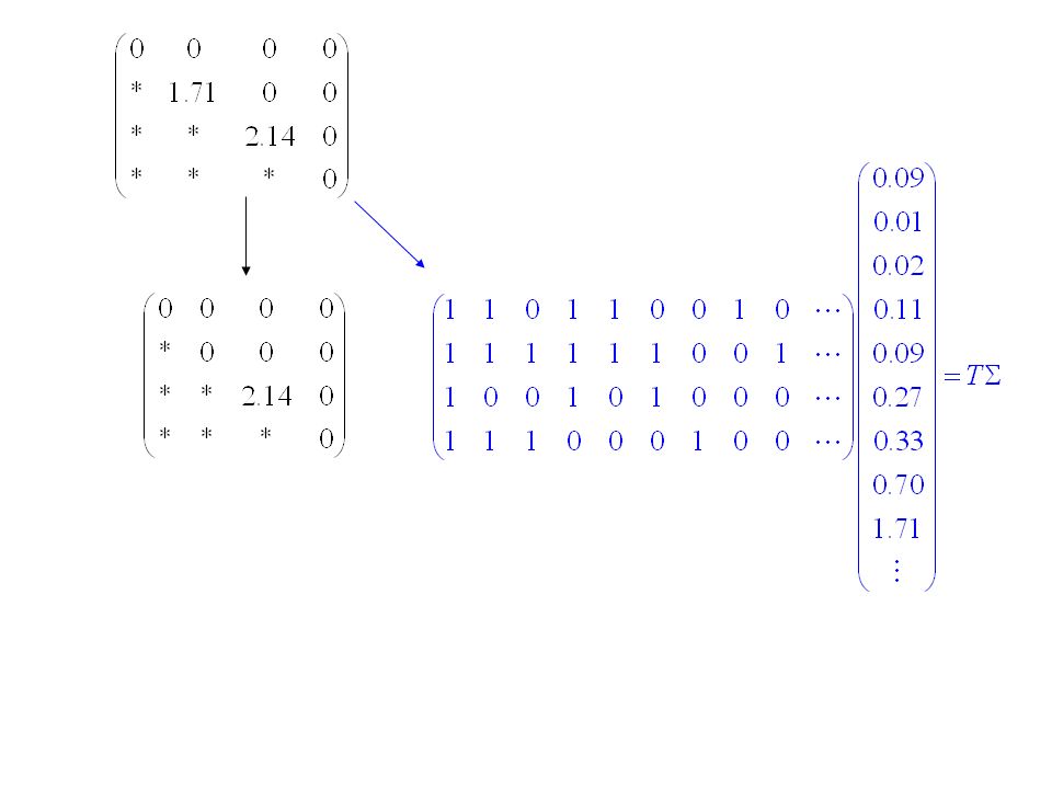
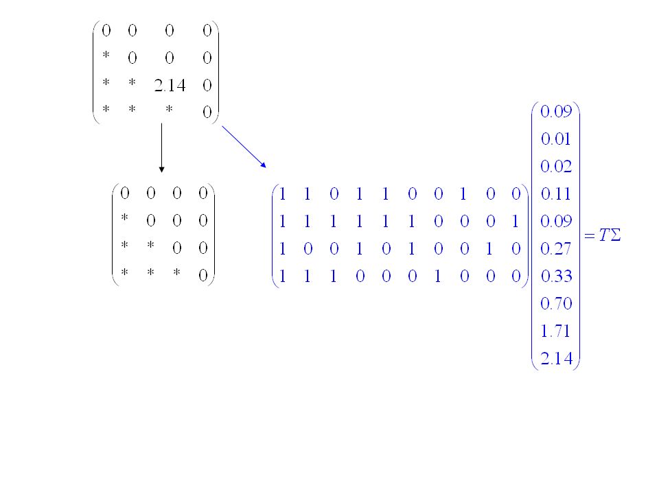
17. Generalizing to n > 2: 1. Park & Shin (1998) algorithm gives variances for X's: Find n  m matrix T consisting of 0’s and 1’s and m-vector such that and 2. Linear programming gives reasonable means for X's: Find m-vector that solves subject to constraints: (i)  i > 0 for all i; and (ii)when  i 2  0.25 3. Generate independent X's with the appropriate distributions and multiply by T: where X is a vector of independent r.v.’s, and T is a matrix of 0’s and 1’s

18. Park & Shin (1998) algorithm gives variances of X's E.g., Suppose for the common component of Y 3 and Y 4

27. Grub population density as a function of several covariates

28. Fitted Values (quartiles) Variance of Residuals 0.5 1.0 1.5 2.0 1st2nd3rd4th 0.0 0.1 0.2 060120 180 Correlation of Residuals Lag distance (feet) Are the conditions for multiple regression met? 1. Non-normal response variable 2. Variance not constant 3. Observations not independent

29. with quasi-likelihood estimation (Wedderburn, 1974) Generalized linear model (Fisher 1935; Dempster 1971; Berk 1972; Nelder and Wedderburn 1972) adapted for spatially dependent observations (Liang and Zeger 1986; McCullagh amd Nelder 1989; Albert and McShane 1995; Gotway and Stroup 1997; Dalthorp 2004 ) A. Accommodates response variables with distribution in exponential family (including normal, binomial, Poisson, gamma, exponential, chi-squared, etc.) B. Allows for non-constant variance A. Accommodates response variables that are not in an exponential family (including negative binomial, unspecified distributions) B. Requires only that the variance of the response variable be expressed as a function of the mean A. Accounts for spatial autocorrelation in the residuals B. The statistical theory for the model is not well-developed

30. Example: Japanese beetle grub population density vs. soil organic matter Organic matter content (%) Grubs per soil sample 3456789 0 2 4 6 Means s2s2 0.0 0.1 0.2 060120 180 Correlation Lag distance (feet) VariancesCorrelations Means (via GLM): Variances (via TPL): Correlations (via spherical model):

31. X’s are independent, count-valued random variables -- variances from Park & Shin’s algorithm -- means from linear programming ### PROBLEM ### No solution found! Choice between one of the following: i. One Y mean off-target but no impossible X r.v.'s Need: Y with  = 0.141 Can only do:  = 0.151 ii. One impossible X r.v. ( ) We need: r.v. with  = 0.0385,  2 = 0.0272 Can do Bernoulli:  = 0.0385,  2 = 0.0370 Consequences? Var(Y 16 ) = 0.139 vs. target of 0.129 The simulation 1000 reps with n = 143:

32. Results for 1000 simulation runs: 3720 X's consisting of: -- Negative binomial: 1580 -- Bernoulli: 2099 -- Bernoulli + Poisson: 40 -- Impossible: 1 (simulated  2 slightly larger than target) Target mean Simulated mean Means Target variance Simulated variance Variances

33. 050100150200250300350400450 -0.05 0 0.05 0.1 0.15 0.2 0.25 Lag distance Correlation Correlations

34. Example: Diamond back moth dispersal Release point Traps Means Variances Mean Variance Lag Distance Correlation 0 0.1 Correlation

35. The simulation 1000 reps with n = 114: X’s are independent negative binomials -- variances from Park & Shin’s algorithm -- means from linear programming T is a matrix of zeros and ones that defines the common components of the Y’s  22 s2s2 Results Means Variances

36. 0510152025303540 -0.05 0 0.05 0.1 0.15 0.2 0.25 Lag distance Correlation Correlation: Simulated vs. target * Circles are averages for 1000 sims

37. Example: Weed counts (Chenopodium polyspermum) vs. soil magnesium Weed counts and soil [Mg] in random quadrats in a field... Means s2s2 Variances

38. Correlation ### Infeasible correlations ### Highest possible correlation between Y i, Y j is: With 49 pairs of points in the weed data, target  i,j is too high.

39. Summary Correlated count r.v.'s can be simulated by overlapping sums of independent negative binomials, Bernoullis, and Poissons The simulated r.v.'s are very close to negative binomial where   2 Negative correlations and strong positive correlations between r.v.’s with very different variances are not attainable, but... The method can accommodate a wide variety of ecologically important scenarios that the hierarchical lognormal-Poisson model balks at, including: -- underdispersed count r.v.'s -- moderately strong correlations where  1   2 and  1 2   2 2