1. Data Needs for Simulations of Electron-driven Processes in Planetary and Cometary Atmospheres by Laurence Campbell & Michael J. Brunger School of Chemical and Physical Sciences, GPO Box 2100, Adelaide, SA 5001, Australia Presented on Wednesday 3 rd October 2012 at ICAMDATA 2012, Gaithersburg, Maryland, USA

2. Aims of our work Inputs required – Atmospheric data – Electron flux spectrum – Electron impact cross sections – Other atomic and molecular dataOutline

3. Aims of our work Inputs required – Atmospheric data – Electron flux spectrum – Electron impact cross sections – Other atomic and molecular data Examples – Electron cooling by CO 2 in the atmosphere of MarsOutline

4. Aims of our work Inputs required – Atmospheric data – Electron flux spectrum – Electron impact cross sections – Other atomic and molecular data Examples – Electron cooling by CO 2 in the atmosphere of Mars – Infrared emissions from CO at Mars and VenusOutline

5. Aims of our work Inputs required – Atmospheric data – Electron flux spectrum – Electron impact cross sections – Other atomic and molecular data Examples – Electron cooling by CO 2 in the atmosphere of Mars – Infrared emissions from CO at Mars and Venus – Predictions of A 1 Π emissions from CO in comet Hale-BoppOutline

6. Aims of our work Inputs required – Atmospheric data – Electron flux spectrum – Electron impact cross sections – Other atomic and molecular data Examples – Electron cooling by CO 2 in the atmosphere of Mars – Infrared emissions from CO at Mars and Venus – Predictions of A 1 Π emissions from CO in comet Hale-Bopp – Electron impact excitation of higher-energy states of O 2 in the atmosphere of EuropaOutline

7. Aims of our work Inputs required – Atmospheric data – Electron flux spectrum – Electron impact cross sections – Other atomic and molecular data Examples – Electron cooling by CO 2 in the atmosphere of Mars – Infrared emissions from CO at Mars and Venus – Predictions of A 1 Π emissions from CO in comet Hale-Bopp – Electron impact excitation of higher-energy states of O 2 in the atmosphere of Europa – Electron heating in the atmosphere of TitanOutline

8. Aims of our work Inputs required – Atmospheric data – Electron flux spectrum – Electron impact cross sections – Other atomic and molecular data Examples – Electron cooling by CO 2 in the atmosphere of Mars – Infrared emissions from CO at Mars and Venus – Predictions of A 1 Π emissions from CO in comet Hale-Bopp – Electron impact excitation of higher-energy states of O 2 in the atmosphere of Europa – Electron heating in the atmosphere of Titan – Emissions from hydrogen at Jupiter ConclusionsOutline

9. Aims To enhance the role of electron-impact cross-section measurements in planetary and cometary modeling by: – Demonstrating the need for more accurate cross sections, as in: electron cooling by CO 2 at Mars, and electron heating at Titan.

10. Aims To enhance the role of electron-impact cross-section measurements in planetary and cometary modeling by: – Demonstrating the need for more accurate cross sections, as in: electron cooling by CO 2 at Mars, and electron heating at Titan. – Encouraging new measurements of required cross sections, as in: electron-driven infrared emissions from CO at Mars and Venus.

11. Aims To enhance the role of electron-impact cross-section measurements in planetary and cometary modeling by: – Demonstrating the need for more accurate cross sections, as in: electron cooling by CO 2 at Mars, and electron heating at Titan. – Encouraging new measurements of required cross sections, as in: electron-driven infrared emissions from CO at Mars and Venus. – Finding applications where electron impact has not been considered previously, such as determination of the abundance of CO in comet Hale-Bopp, and excitation of the higher-energy states of O 2 at Europa.

12. Electron cooling and heating Electron cooling – thermal electrons lose energy by vibrational excitation of molecules Energy Time Electron impact excitation Electron cooling

13. Electron cooling and heating Electron cooling – thermal electrons lose energy by vibrational excitation of molecules Radiative decay – polar molecules (CO, CO 2 ) radiate heat to space Energy Time Electron impact excitation Radiative Decay Electron cooling Energy lost from atmosphere

14. Electron cooling and heating Electron cooling – thermal electrons lose energy by vibrational excitation of molecules Radiative decay – polar molecules (CO, CO 2 ) radiate heat to space Electron heating – for N 2, the vibrational energy is transferred to heat of neutral species in collisions Energy Time Electron impact excitation Radiative Decay Collisional quenching Electron cooling Electron heating (of atmosphere) Energy lost from atmosphere

15. We determine (from measurements or theory) a flux distribution F(E) i.e. the number of electrons of energy E crossing a unit area in unit time. Electron cooling rate

16. We determine (from measurements or theory) a flux distribution F(E) i.e. the number of electrons of energy E crossing a unit area in unit time. The flux distribution is folded with the Integral Cross Section σ 0ν (E) for vibrational excitation from ground to level ν to give the electron energy transfer rate Q 0 : Electron cooling rate

17. We determine (from measurements or theory) a flux distribution F(E) i.e. the number of electrons of energy E crossing a unit area in unit time. The flux distribution is folded with the Integral Cross Section σ 0ν (E) for vibrational excitation from ground to level ν to give the electron energy transfer rate Q 0 : Electron cooling rate Electron cooling rate =

18. CO 2 electron impact excitation cross sections Present ICS ( ) and ICS used by Morrison and Greene, 1978 ( )

19. Mars - Calculated electron cooling by CO 2 Using cross sections of Morrison and Green, 1978 ( ) for average electron density.

20. Using current cross sections for ( ) Average electron density (- - - - -) Minimum electron density ( ) Maximum electron density Demonstrates importance of accurate electron-impact cross sections in planetary studies. Mars - Calculated electron cooling by CO 2

21. CO vibrational cross sections Measurements of electron- impact vibrational cross sections for excitation of CO by: (— - —) Poparić et al., 2006, scaled to Gibson et al., 1996 ( ☐ ) ( ) Allan, 2010 (- - - - -) Extrapolated

22. Mars daytime CO infrared emissions Comparing (1→0) and (2→1) emissions for:  Electron-impact (- - - -)  Fluorescence and photolysis ( )

23. Mars daytime CO infrared emissions Comparing (1→0) and (2→1) emissions for:  Electron-impact (- - - -)  Fluorescence and photolysis ( ) Electron impact is significant above  180 km for (1→0) emissions.

24. Venus daytime CO infrared emissions Comparing (2→1) emissions for: Sunlight ( ) Thermal + auroral ( ☐ ) Photoelectrons ( ) Comparing (3→2) emissions for: Sunlight (- - - - -) Thermal + auroral () Photoelectrons (  ) Electron-impact is significant above 190 km for (3→2) emissions.

25. Venus daytime CO infrared emissions Comparing (2→1) emissions for: Sunlight ( ) Thermal + auroral ( ☐ ) Photoelectrons ( ) Comparing (3→2) emissions for: Sunlight (- - - - -) Thermal + auroral () Photoelectrons (  ) Electron-impact is significant above 190 km for (3→2) emissions. Photoelectron impact is significant at 250 km for (2→1) emissions.

26. A spectrum ( ) of emissions from the coma of comet Hale-Bopp. The authors superimposed a fitted spectrum ( ) of the fourth positive (A 1  X 1  + ) band emissions of CO, from which they determined the abundance of CO in the coma. It was assumed that the CO emissions were due to fluorescence induced by sunlight, without any contribution from photoelectron impact. Observed Fitted CO O I lines Fitted S I lines CO in comet Hale-Bopp

27. A spectrum ( ) of emissions from the coma of comet Hale-Bopp. The authors superimposed a fitted spectrum ( ) of the fourth positive (A 1  X 1  + ) band emissions of CO, from which they determined the abundance of CO in the coma. It was assumed that the CO emissions were due to fluorescence induced by sunlight, without any contribution from photoelectron impact. Observed Fitted CO O I lines Fitted S I lines CO in comet Hale-Bopp

28. Recent cross sections Cross section examples and comparison with theory =0 CO A 1 

29. Recent cross sections Cross section examples and comparison with theory CO A 1 

30. We find that electron impact ( ) makes a substantial contribution, thus reducing the implied amount of fluorescence ( ). Hence the implied CO abundance is reduced by 40%. CO in comet Hale-Bopp

31. O 2 - Measurements at Sophia – sample energy loss spectrum

32. Measurements – Integral cross sections (  ) Measurements

33. Measurements – Integral cross sections (  ) Measurements ( ) BEf-scaled predictions (Suzuki et al., 2010)

34. Measurements – Integral cross sections (  ) Measurements ( ) BEf-scaled predictions (Suzuki et al., 2010) ( ) Adjusted cross sections are used for the longest band.

35. Measurements – Integral cross sections (  ) Measurements ( ) BEf-scaled predictions (Suzuki et al., 2010) ( ) Adjusted cross sections are used for the longest band. ( ) Previous measurements (Shyn et al., 1994)

36. Decay and predissociation Radiative decay only for vibrational levels below 7.01 eV

37. Decay and predissociation Radiative decay only for vibrational levels below 7.01 eV Excitation results in predissociation above 7.01 eV

38. Decay and predissociation Radiative decay only for vibrational levels below 7.01 eV Excitation results in predissociation above 7.01 eV Measurements of predissociation channels by Stephen Gibson: ( ) O 2  O( 1 D)+O( 3 P) ( ) O 2  O( 3 P)+O( 3 P)

39. ground O 2 SR(r) O 2 LB O 2 SB Time (schematic) Excitation Atomic and molecular processes

40. ground O( 1 D) O 2 SR(r) O 2 LB O 2 SB Time (schematic) Predissociation Excitation Atomic and molecular processes

41. ground O( 1 D) O 2 SR(r) O 2 LB O 2 SB Time (schematic) Predissociation Excitation Quenching Atomic and molecular processes

42. ground O( 1 D) O 2 SR(r) O 2 LB O 2 SB Time (schematic) Predissociation Excitation Radiation Quenching Atomic and molecular processes

43. ground O( 1 D) O( 1 S) O 2 SR(r) O 2 LB O 2 SB Time (schematic) Predissociation Excitation Radiation Quenching Atomic and molecular processes

44. ground O( 1 D) O( 1 S) O 2 SR(r) O 2 LB O 2 SB O2+O2+ Time (schematic) Predissociation Ionisation Excitation Radiation Quenching Atomic and molecular processes

45. ground O( 1 D) O( 1 S) O 2 SR(r) O 2 LB O 2 SB O2+O2+ Time (schematic) Predissociation Recombination Ionisation Excitation Radiation Quenching

46. Electron flux spectrum for Europa Secondary electrons Magnetospheric flux

47. Electron flux spectrum for Europa Secondary electrons Magnetospheric flux

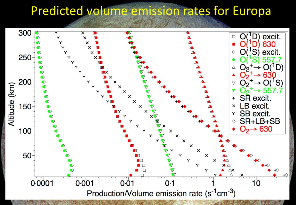
48. Predicted volume emission rates for Europa

51. Predicted 630.0-nm/557.7-nm ratio for Europa The predicted ratio of the 630.0-nm to 557.7-nm intensities is shown as a function of altitude in the atmosphere of Europa, for: (----) excitation of O atoms and recombination of O 2 +. ( ) as above, plus excitation of the Schumann-Runge continuum, longest band and second band of O 2.

52. Previous study Electron impact excitation (  ) Radiative transitions (  ) Titan – range of processes in N 2 Previous study

53. Titan – range of processes in N 2 Previous study (lower) and updated study (upper). Electron impact excitation (  ) Radiative transitions (  or |) Predissociation (  ) Quenching (  ) Previous study

54. Titan – Electron heating Previous study (lower) and updated study (upper). Electron impact excitation (  ) Radiative transitions (  or |) Predissociation (  ) Quenching (  ) Electron heating ( ) Previous study

55. Energy Excitation State X State  Statistical equilibrium - solve simultaneous continuity equations until: population(  ) x loss rate = total gain of  State  i Statistical-equilibrium calculation

56. Energy Excitation Radiative Decay State X State  Statistical equilibrium - solve simultaneous continuity equations until: population(  ) x loss rate = total gain of  State  i Statistical-equilibrium calculation

57. Energy Excitation Radiative Decay State X State  Statistical equilibrium - solve simultaneous continuity equations until: population(  ) x loss rate = total gain of  State  i Statistical-equilibrium calculation State γ j

58. Energy Excitation Radiative Decay State X State  Statistical equilibrium - solve simultaneous continuity equations until: population(  ) x loss rate = total gain of  State  i Quenching (electron heating) Statistical-equilibrium calculation State γ j

59. Previous and current N 2 cross sections In previous calculations old N 2 cross sections (left) were used. We have repeated the calculations using more recent (right) cross sections.

60. Titan – electron heating rates Previous study: −Electronic states − Vibrational ( ν =1)

61. Titan – electron heating rates Previous study: −Electronic states − Vibrational ( ν =1) Emulation of previous study: ▲ Electronic states ♦ Vibrational

62. Titan – electron heating rates Previous study: −Electronic states − Vibrational ( ν =1) Emulation of previous study: ▲ Electronic states ♦ Vibrational New study: Vibrational ( ν =1)

63. Titan – electron heating rates Previous study: −Electronic states − Vibrational ( ν =1) Emulation of previous study: ▲ Electronic states ♦ Vibrational New study: Vibrational ( ν =1) △ Electronic states ♢ Vibrational ( ν =1-10)

64. Titan- data needs for improved calculation Measurements of collision-induced electronic transitions (CIETs)  for verification of recent theoretical values by Kirillov, 2012.

65. Titan- data needs for improved calculation Measurements of collision-induced electronic transitions (CIETs)  for verification of recent theoretical values by Kirillov, 2012. Electron-impact excitation cross sections for higher-energy excited states of N 2. (New measurements by Kato et al., 2010 and Khakoo et al., 2008).  Predissociation, radiative-transition and quenching probabilities of these states.

66. Titan- data needs for improved calculation Measurements of collision-induced electronic transitions (CIETs)  for verification of recent theoretical values by Kirillov, 2012. Electron-impact excitation cross sections for higher-energy excited states of N 2. (New measurements by Kato et al., 2010 and Khakoo et al., 2008).  Predissociation, radiative-transition and quenching probabilities of these states. Reaction rates for excited N 2 e.g. N 2 [A 3 Σ u + ] + O  NO + N( 2 D).  Update of values by Herron, 1999 and Kochetov et al., 1987.

67. Titan- data needs for improved calculation Measurements of collision-induced electronic transitions (CIETs)  for verification of recent theoretical values by Kirillov, 2012. Electron-impact excitation cross sections for higher-energy excited states of N 2. (New measurements by Kato et al., 2010 and Khakoo et al., 2008).  Predissociation, radiative-transition and quenching probabilities of these states. Reaction rates for excited N 2 e.g. N 2 [A 3 Σ u + ] + O  NO + N( 2 D).  Update of values by Herron, 1999 and Kochetov et al., 1987. Electron-impact excitation cross sections for CH 4. Rates for vibrational-vibrational (VV) and vibrational- translational (VT) interactions between CH 4 and N 2.

68. Jupiter – Lyman-α emissions Two electron impact processes: Direct excitation: e + H(1s)  e + H(2p)  H(1s) + Lyman-α (using CCC calculation, Zammit, 2010)

69. Jupiter – Lyman-α emissions Two electron impact processes: Direct excitation: e + H(1s)  e + H(2p)  H(1s) + Lyman-α (using CCC calculation, Zammit, 2010) Impact dissociation of H 2 : e + H 2  e + H(2p) + H(nl)  H(1s) + Lyman-α (using emission cross sections from Tawara et al., 1990) As cross sections of similar shape, Lyman-α emission profile is mainly a function of the ratio of H to H 2.

70. Jupiter – Lyman-α emissions Two electron impact processes: Direct excitation: e + H(1s)  e + H(2p)  H(1s) + Lyman-α (using CCC calculation, Zammit, 2010) Impact dissociation of H 2 : e + H 2  e + H(2p) + H(nl)  H(1s) + Lyman-α (using emission cross sections from Tawara et al., 1990) As cross sections of similar shape, Lyman-α emission profile is mainly a function of the ratio of H to H 2. Data needs: Verification of emission cross sections.

71. Conclusions Recent measurements of electron impact cross sections have: – led to new applications, such as calculations of: emissions from CO in comet Hale-Bopp, infrared emissions from CO at Mars and Venus, and the intensity ratio 630.0-nm/557.7-nm at Europa. – Enabled more accurate calculations, such as of: electron cooling at Mars and electron heating rates at Titan. Often these calculations require a wide range of data for subsequent processes, including radiative transitions, quenching rates, VV and VT interactions, CIET rates and chemical reactions. Acknowledgements This work was supported by the Australian Research Council through its Centres of Excellence Program. Michael Brunger thanks the University of Malaya for his “Distinguished Visiting Professor” appointment.

72. CO cooling rates - Mars Calculated electron cooling rates by CO at Mars using cross sections of: for 0  ν =1, ( ) Allan, 1989 (— —) Poparić et al., 2006 (- - - - - -) Allan, 2010 for sum of 0  ν =2,3,…,10, (-  -  -  -  -) Allan, 1989 (      ) Poparić et al., 2006 ( ) Allan, 2010