1. 13
EXPENDITURE MULTIPLIERS: THE KEYNESIAN MODEL
CHAPTER

2. Objectives After studying this chapter, you will able to
Explain how expenditure plans and real GDP are determined when the price level is fixed
Explain the expenditure multiplier
Explain how recessions and expansions begin
Explain the relationship between aggregate expenditure and aggregate demand
Explain how the multiplier gets smaller as the price level changes

3. Economic Amplifier or Shock Absorber?
A voice can be a whisper or fill Central Park, depending on the amplification.
A limousine with good shock absorbers can ride smoothly over terrible potholes.
Investment and exports can fluctuate like the amplified voice, or the terrible potholes; does the economy react like a limousine, smoothing out the bumps, or like an amplifier, magnifying the fluctuations?
These are the questions this chapter addresses.

4. Fixed Prices and Expenditure Plans
The Aggregate Implications of Fixed Prices
In the very short run, prices are fixed and the aggregate amount that is sold depends only on the aggregate demand for goods and services.
In this very short run, to understand real GDP fluctuations, we must understand aggregate demand fluctuations.

5. Fixed Prices and Expenditure Plans
The four components of aggregate expenditure—consumption expenditure, investment, government purchases of goods and services, and net exports—sum to real GDP.
Aggregate planned expenditure equals planned consumption expenditure plus planned investment plus planned government purchases plus planned exports minus planned imports.

6. Fixed Prices and Expenditure Plans
A two-way link exists between aggregate expenditure and real GDP
An increase in real GDP increases aggregate expenditure
An increase in aggregate expenditure increases real GDP

7. Fixed Prices and Expenditure Plans
Consumption Function and Saving Function
Consumption and saving are influenced by
The real interest rate
Disposable income
Wealth
Expected future income.
Disposable income is aggregate income (GDP) minus taxes plus transfer payments.
The consumption function and saving function. In Chapter 23, the student learned about the influences on saving. They learned there that households divide their disposable income between consumption expenditure and saving. And they learned that the factors that affect saving are the real interest rate, disposable income, wealth, and expected future income. These same ideas repeat in this chapter but with a different emphasis. Be sure that the students see that they are talking about exactly the same stuff by they are looking at it from a different angle. In Chapter 23, the focus was on the saving part of the allocation; here it is primarily on the consumption part. In Chapter 23, we held disposable income constant and studied the saving supply curve—the relationship between saving and the real interest rate, other things remaining the same. Here, we hold the real interest rate constant and study the saving and consumption functions—the relationships between saving (and consumption) and disposable income, other things remaining the same.
An analogy might help. Ask the students if they have ever been to a ball game (could be any fast-moving game) and disagreed with a referee’s (or umpire’s) ruling. Almost everyone has. Both the referee and the spectator were at the same event, but they viewed it from a different angle. That’s what we’re doing here. We’ve viewing the allocation of disposable income between saving and consumption from a different angle. But we’re at the same ball game that we were at in Chapter 23.

8. Fixed Prices and Expenditure Plans
To explore the two-way link between real GDP and planned consumption expenditure, we focus on the relationship between consumption expenditure and disposable income when the other factors are constant.
The relationship between consumption expenditure and disposable income, other things remaining the same, is the consumption function.
And the relationship between saving and disposable income, other things remaining the same, is the saving function.

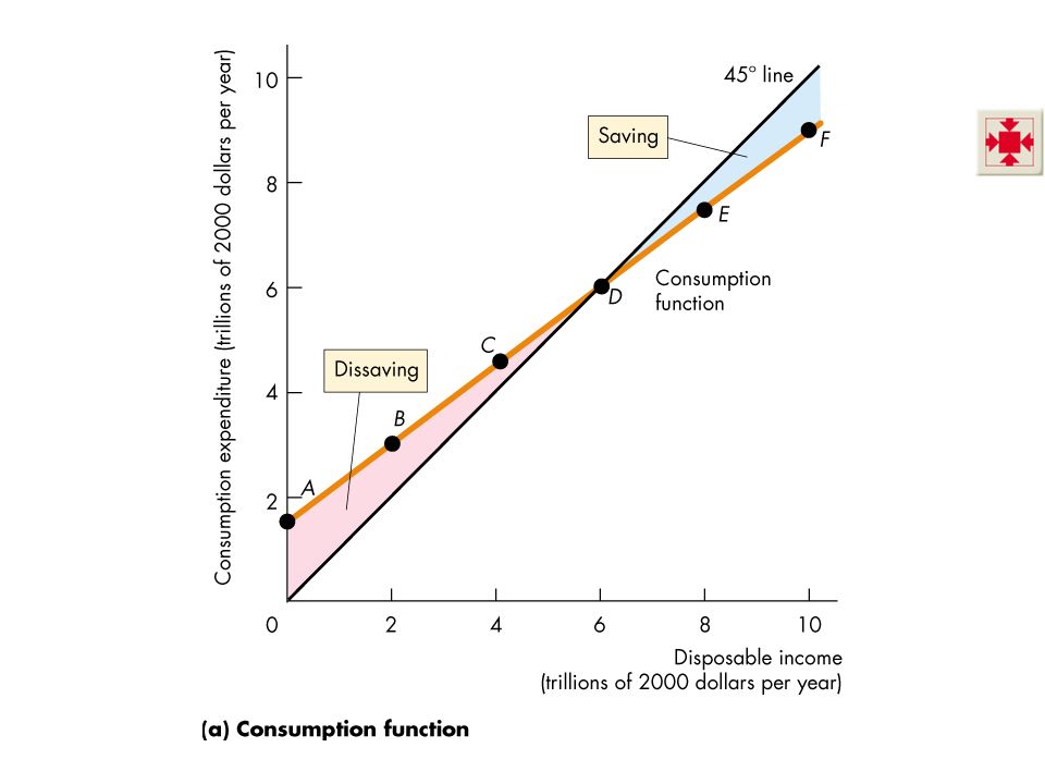
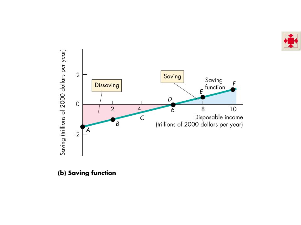
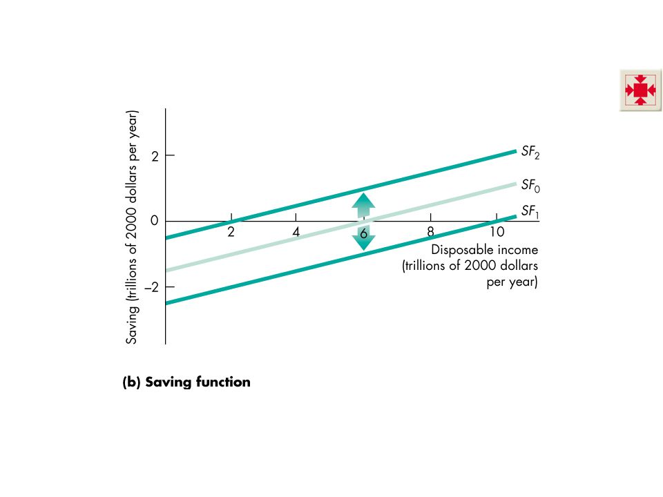
9. Fixed Prices and Expenditure Plans
Figure 29.1 illustrates the consumption function and the saving function.
The 45° line. Don’t assume that the student immediately understands the 45° line! Spend a bit of time explaining how to “read” it. Fundamentally, the line is that along which x = y. This line happens to be a 45° line when the scales along the x-axis and the y- axis are the same. Then point out that the horizontal distance to a point along the x-axis equals the vertical distance from that point to the 45° line. So at all points along the 45° line, x = y. If you wish, you can go on to show the students how the x = y line changes its appearance if we stretch or squeeze the scale on the y-axis holding the scale on the x-axis constant. Emphasize that x and y can be anything. In Figure 29.1, x is disposable income and y is consumption expenditure; in Figure 29.6(a), x is real GDP and y is aggregate planned expenditure.

12. Fixed Prices and Expenditure Plans
Marginal Propensities to Consume and Save
The marginal propensity to consume (MPC) is the fraction of a change in disposable income spent on consumption.
It is calculated as the change in consumption expenditure, C, divided by the change in disposable income, YD, that brought it about.
That is:
MPC = C/YD
Marginal and average propensities. The text defines the MPC and MPS, and shows that they sum to one because disposable income can only be consumed or saved.
The textbook does not define and explain the APC and APS. The reason is that these concepts have no operational significance. They are not worth any of the student’s attention.

13. Fixed Prices and Expenditure Plans
The marginal propensity to save (MPS) is the fraction of a change in disposable income that is saved.
It is calculated as the change in saving, S, divided by the change in disposable income, YD, that brought it about.
That is:
MPS = S/YD

14. Fixed Prices and Expenditure Plans
The MPC plus the MPS equals one.
To see why, note that,
C + S = YD.
Divide this equation by YD to obtain,
C/YD + S/YD = YD/YD, or
MPC + MPS = 1.

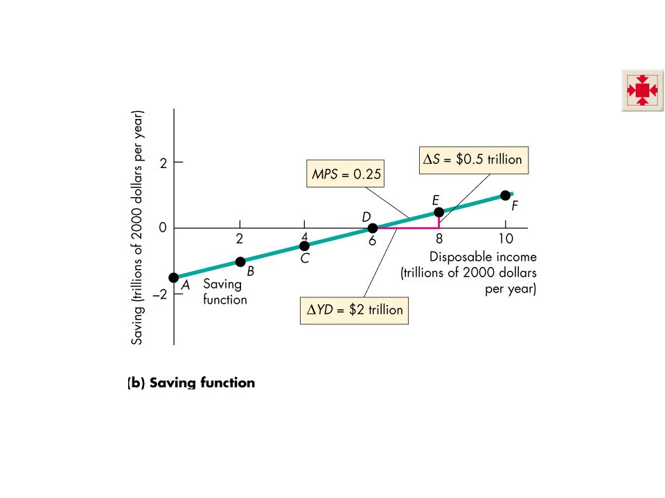
15. Fixed Prices and Expenditure Plans
Slopes and Marginal Propensities
Figure 29.2 shows that the MPC is the slope of the consumption function and the MPS is the slope of the saving function.

18. Fixed Prices and Expenditure Plans
Other Influences on Consumption Expenditure and Saving
When an influence other than disposable income changes—the real interest rate, wealth, or expected future income—the consumption function and saving function shift.
Figure 29.3 illustrates these effects.

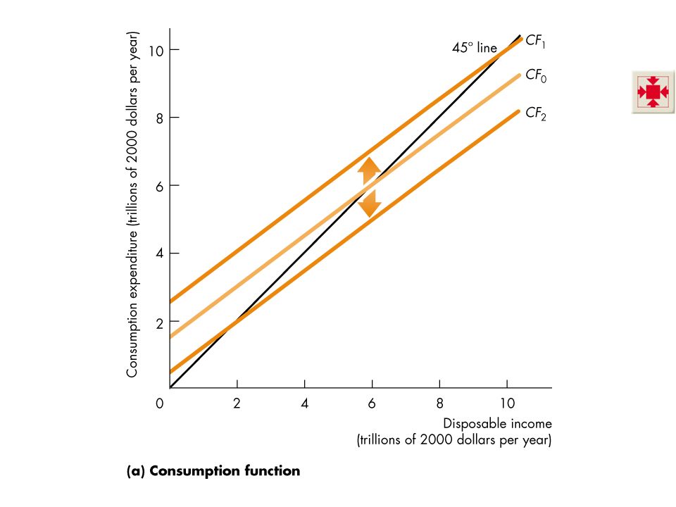
21. Fixed Prices and Expenditure Plans
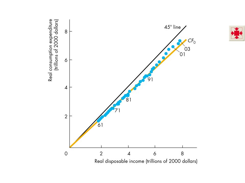
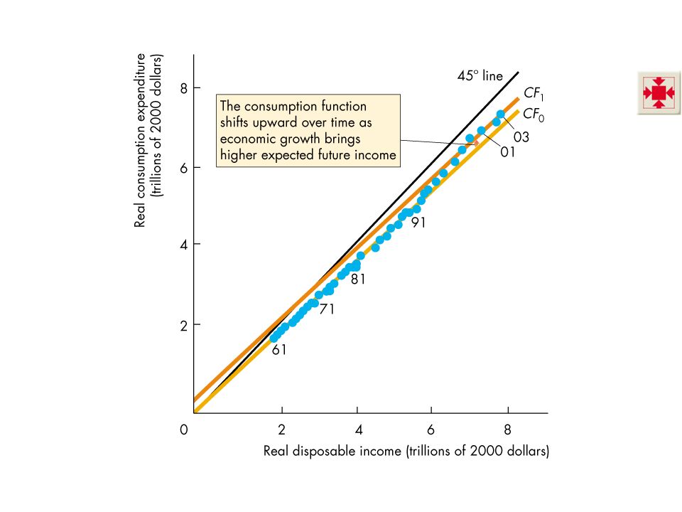
The U.S. Consumption Function
In 1961, the U.S. consumption function was CF0.
The dots show consumption and disposable income for each year from 1961 to 2003.

23. Fixed Prices and Expenditure Plans
The consumption function has shifted upward over time because economic growth has created greater wealth and higher expected future income.
The assumed MPC in the figure is 0.9.

25. Fixed Prices and Expenditure Plans
Consumption as a Function of Real GDP
Disposable income changes when either real GDP changes or when net taxes change.
If tax rates don’t change, real GDP is the only influence on disposable income, so consumption expenditure is a function of real GDP.
We use this relationship to determine equilibrium expenditure.

26. Fixed Prices and Expenditure Plans
Import Function
In the short run, imports are influenced primarily by U.S. real GDP.
The marginal propensity to import is the fraction of an increase in real GDP spent on imports.
In recent years, NAFTA and increased integration in the global economy have increased U.S. imports.
Removing the effects of these influences, the U.S. marginal propensity to import is probably about 0.2.

27. Real GDP with a Fixed Price Level
The relationship between aggregate planned expenditure and real GDP can be described by an aggregate expenditure schedule, which lists the level of aggregate expenditure planned at each level of real GDP.
The relationship can also be described by an aggregate expenditure curve, which is a graph of the aggregate expenditure schedule.
Historical background. If you want to talk about Keynes and his contribution to economics, this is probably the best place to do it. The part closer (pp. 497–502 in Economics or pp. 151–156 in Macroeconomics) provides a brief biography of Keynes and sketches the essence of the distinction between Says Law and Keynes principle of effective demand. A more comprehensive Keynes biographical sketch can be found at
The model, now generally called the aggregate expenditure model, presented in this section is the essence of Keynes General Theory. According to Don Patinkin, a leading historian of economic thought and Keynes scholar says that the innovation of the General Theory was to replace price with income (GDP) as the equilibrating variable. This version of the model cannot be found in the General Theory, mainly because Keynes was writing before the national income accounting system had been developed. So he made up his own aggregates, based on employment and a money wage measure of the price level. But the words and equations of the General Theory can be translated readily into the textbook version of the model. This version of the model first appeared in The Elements of Economics, a textbook authored by Lorie Tarshis published in It was popularized by Paul Samuelson in the first edition of his celebrated text published in 1948.
[continued on notes page for next slide]

28. Real GDP with a Fixed Price Level
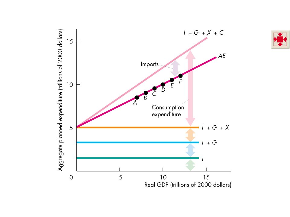
Aggregate Planned Expenditure and Real GDP
Figure 29.5 shows how the aggregate expenditure curve is built from its components.
The main difference between the Keynesian cross model of the 1940s and the aggregate expenditure model of today is that from the 1940s through the mid-1960s, economists believed that the fixed price level assumption was an acceptable (if not exactly accurate) description of reality, so the model was seen as actually determining real GDP, and the multiplier was seen as an empirically relevant phenomenon. In contrast, today, we see the model as part of the aggregate demand story. The value of the model today—and it is valuable today and not, as some people claim, eclipsed by the AS-AD model and irrelevant—is that it explains the multiplier that translates a change in autonomous expenditure into a shift of the AD curve and it explains the multiplier convergence process that pulls the economy toward the AD curve. (When an unintended change in inventories occurs, the economy is off the AD curve but moving toward it.)

30. Real GDP with a Fixed Price Level
Consumption expenditure minus imports, which varies with real GDP, is induced expenditure.
The sum of investment, government purchases, and exports, which does not vary with GDP, is autonomous expenditure.
Consumption expenditure and imports can have an autonomous component.

31. Real GDP with a Fixed Price Level
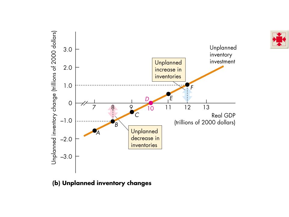
Actual Expenditure, Planned Expenditure, and Real GDP
Actual aggregate expenditure is always equal to real GDP.
Aggregate planned expenditure may differ from actual aggregate expenditure because firms can have unplanned changes in inventories.

32. Real GDP with a Fixed Price Level
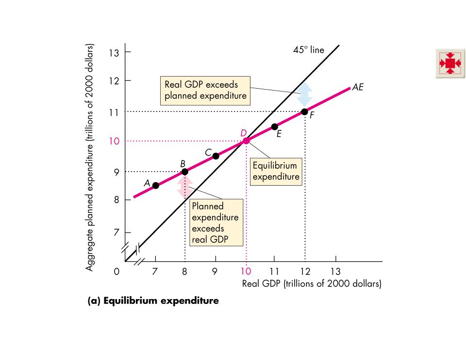
Equilibrium Expenditure
Equilibrium expenditure is the level of aggregate expenditure that occurs when aggregate planned expenditure equals real GDP.

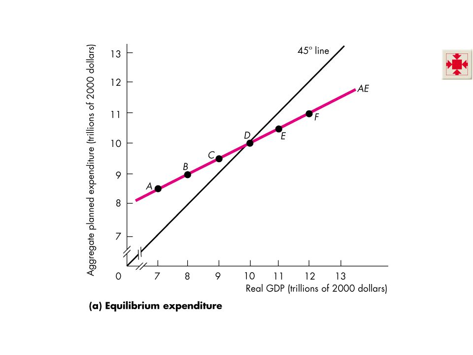
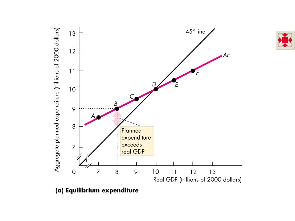
33. Real GDP with a Fixed Price Level
Figure 29.6 illustrates equilibrium expenditure, which occurs at the point at which the aggregate expenditure curve crosses the 45° line and there are no unplanned changes in business inventories.

36. Real GDP with a Fixed Price Level
Convergence to Equilibrium
Figure 29.6 also illustrates the process of convergence toward equilibrium expenditure.
Convergence toward equilibrium. The treatment of the aggregate expenditure model in this textbook plays up Patinkin’s modern interpretation the role of changes in income signaled by unintended inventory changes, as the force that generates equilibrium expenditure.
Figure 29.5 that generates the AE curve and Figure 29.6 that explains convergence toward equilibrium are the core of the model.

39. Real GDP with a Fixed Price Level
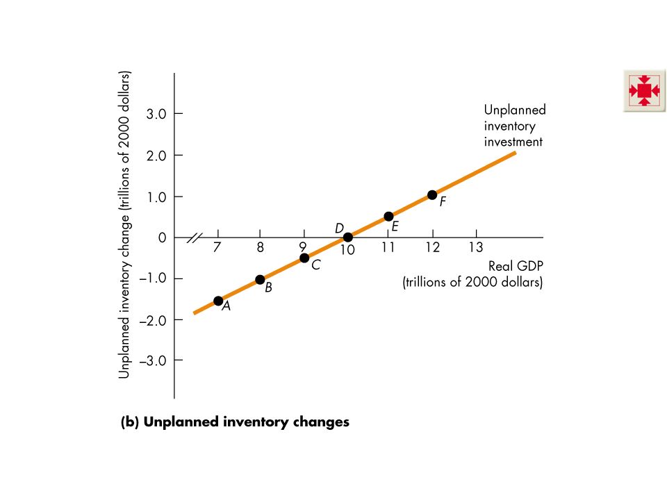
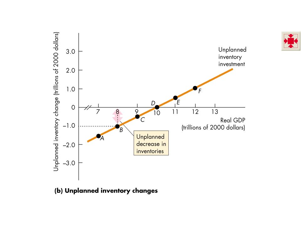
If aggregate planned expenditure is greater than real GDP (the AE curve is above the 45° line), an unplanned decrease in inventories induces firms to hire workers and increase production, so real GDP increases.

42. Real GDP with a Fixed Price Level
If aggregate planned expenditure is less than real GDP (the AE curve is below the 45° line), an unplanned increase in inventories induces firms to fire workers and decrease production, so real GDP decreases.

45. Real GDP with a Fixed Price Level
If aggregate planned expenditure equals real GDP (the AE curve intersects the 45° line), no unplanned changes in inventories occur, so firms maintain their current production and real GDP remains constant.

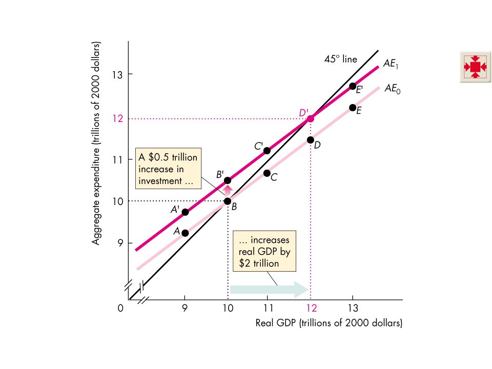
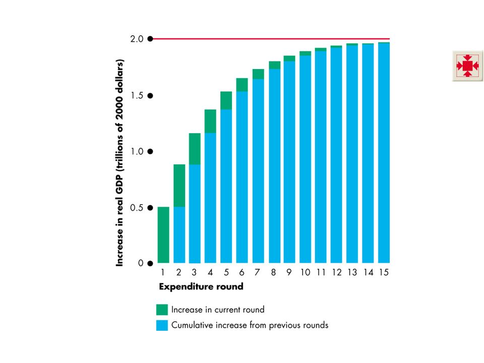
48. The Multiplier
The multiplier is the amount by which a change in autonomous expenditure is magnified or multiplied to determine the change in equilibrium expenditure and real GDP.
The basic idea and practice. Students need quite a lot of practice using multipliers. One good problem involves working out the effects on consumption as well as GDP of a change in investment (when the price level is fixed). The best way to present this problem to the students seems to be sequentially. Begin by giving them the data necessary to deduce how real GDP changes from an increase in investment. Tell them there is no foreign trade, so that there are no exports or imports, and no income taxes. Tell them that the marginal propensity to consume is b (pick any valid number you like), and that investment has changed by ∆I (pick any valid number you like).
Then, after the students have computed the change in GDP, ask them what the change in consumption expenditure is.
Review their attempts to answer this question as follows: The change in GDP, ∆Y, is given by the equation: ∆Y = ∆C + ∆I. Given ∆I from the initial statement of the problem and ∆Y from the first set of calculations, the students can readily calculate ∆C. Focusing the students’ attention on the change in consumption is important because it reinforces the point that a change in autonomous expenditure (investment in this example) leads to an induced change in consumption expenditure and that this increase in consumption expenditure is the source of the multiplier.
The multiplier and the circular flow. Some instructors like to illustrate the multiplier, and give context to Figure 29.8, by using a circular flow diagram to trace out the effect round by round of an initial change in autonomous expenditure. If you do this exercise, use the concrete numbers of Figure 29.8 and initially omit consideration of government and the rest of the world.

49. The Multiplier The Basic Idea of the Multiplier
An increase in investment (or any other component of autonomous expenditure) increases aggregate expenditure and real GDP and the increase in real GDP leads to an increase in induced expenditure.
The increase in induced expenditure leads to a further increase in aggregate expenditure and real GDP.
So real GDP increases by more than the initial increase in autonomous expenditure.

50. The Multiplier Figure 29.7 illustrates the multiplier.
The Multiplier Effect
The amplified change in real GDP that follows an increase in autonomous expenditure is the multiplier effect.

52. The Multiplier
When autonomous expenditure increases, inventories make an unplanned decrease, so firms increase production and real GDP increases to a new equilibrium.

54. The Multiplier Why Is the Multiplier Greater than 1?
The multiplier is greater than 1 because an increase in autonomous expenditure induces further increases in expenditure.
The Size of the Multiplier
The size of the multiplier is the change in equilibrium expenditure divided by the change in autonomous expenditure.

55. The Multiplier
The Multiplier and the Marginal Propensities to Consume and Save
Ignoring imports and income taxes, the marginal propensity to consume determines the magnitude of the multiplier.
The multiplier equals 1/(1 – MPC) or, alternatively, 1/MPS.

56. The Multiplier
Figure 29.8 illustrates the multiplier process and shows how the MPC determines the magnitude of the amount of induced expenditure at each round as aggregate expenditure moves toward equilibrium expenditure.

58. The Multiplier Math ∆Y = ∆I + b∆I + b2∆I + b3∆I + b4∆I + b5∆I + ….
Multiply by b to obtain
b∆Y = b∆I + b2∆I + b3∆I + b4∆I + b5∆I + ….
bn approaches zero as n becomes large so b(n + 1) also approaches zero.
Subtract the second equation from the first to obtain
∆Y – b∆Y = ∆I, or (1 – b) ∆Y = ∆I,
so that
∆Y = ∆I/(1 – b).
The math of the multiplier process. Some instructors like to illustrate that the multiplier is the sum of the increments at each “round” in the multiplier process. This illustration teaches the student the neat facts about the sum of a convergent geometric series.
[To use this slide, unhide it by clicking Slide Show, Hide Slide]

59. The Multiplier Imports and Income Taxes
Income taxes and imports both reduce the size of the multiplier.
Including income taxes and imports, the multiplier equals 1/(1 – slope of the AE curve).
The general multiplier with taxes and foreign trade. You might want provide a more thorough and detailed derivation of the general multiplier formula, which the textbook presents in its simplest form as “one divided by one minus the slope of the AE curve” To do so, you can use the math note on pp. 598–599 (macro 252–253) and show your students that the slope of the AE curve is [b(1 – t) – m] so that the multiplier is .1/[1 – b(1 – t) + m].

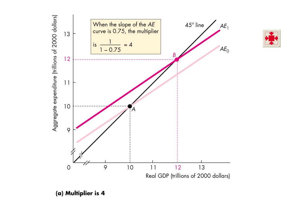
60. The Multiplier
Figure 29.9 shows the relation between the multiplier and the slope of the AE curve.
In part (a) the slope of the AE curve is 0.75 and the multiplier is 4.

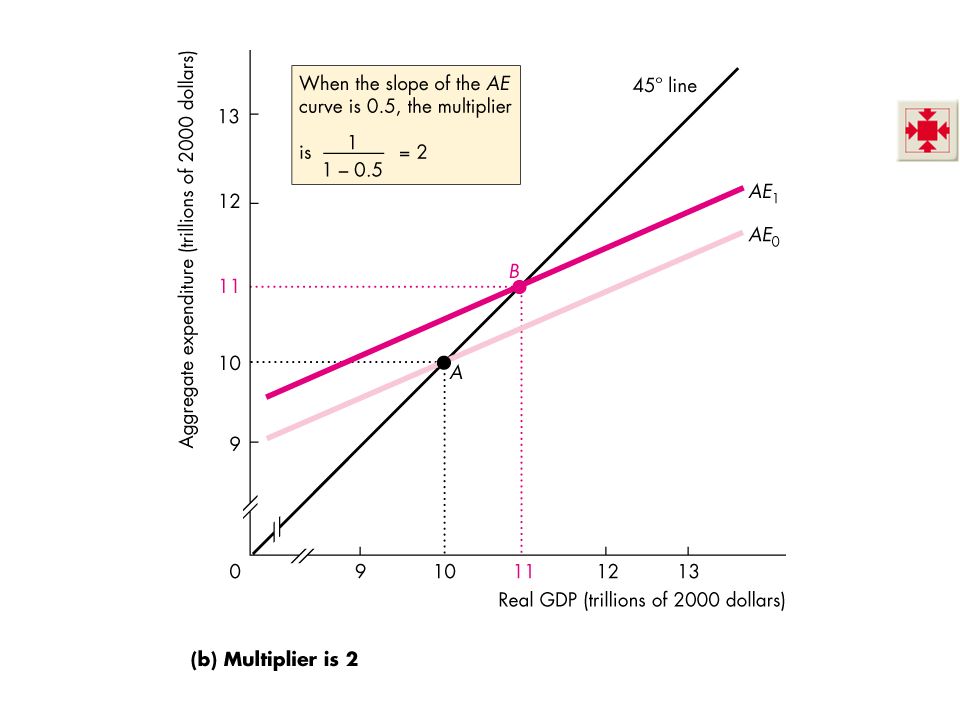
62. The Multiplier
In part (b) the slope of the AE curve is 0.5 and the multiplier is 2.

64. The Multiplier Business Cycle Turning Points
Turning points in the business cycle—peaks and troughs—occur when autonomous expenditure changes.
An increase in autonomous expenditure brings an unplanned decrease in inventories, which triggers an expansion.
A decrease in autonomous expenditure brings an unplanned increase in inventories, which triggers a recession.

65. The Multiplier and the Price Level
In the equilibrium expenditure model, the price level is constant.
But real firms don’t hold their prices constant for long.
When they have an unplanned change in inventories, they change production and prices.
And the price level changes when firms change prices.
The aggregate supply-aggregate demand model explains the simultaneous determination of real GDP and the price level.
The two models are related.

66. The Multiplier and the Price Level
Aggregate Expenditure and Aggregate Demand
The aggregate expenditure curve is the relationship between aggregate planned expenditure and real GDP, with all other influences on aggregate planned expenditure remaining the same.
The aggregate demand curve is the relationship between the quantity of real GDP demanded and the price level, with all other influences on aggregate demand remaining the same.

67. The Multiplier and the Price Level
Aggregate Expenditure and the Price Level
When the price level changes, a wealth effect and substitution effect change aggregate planned expenditure and change the quantity of real GDP demanded.
Figure on the next slide illustrates the effects of a change in the price level on the AE curve, equilibrium expenditure, and the quantity of real GDP demanded.

68. The Multiplier and the Price Level
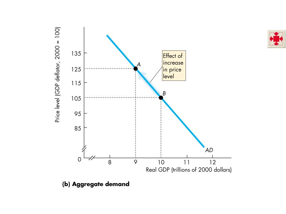
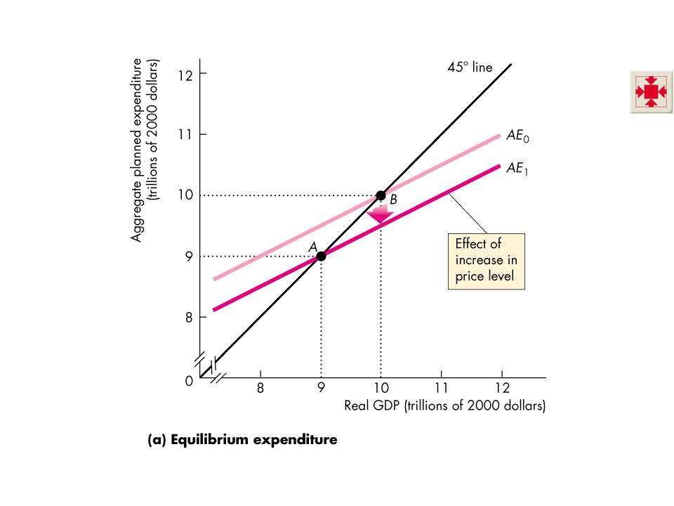
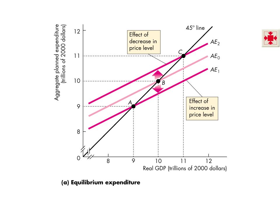
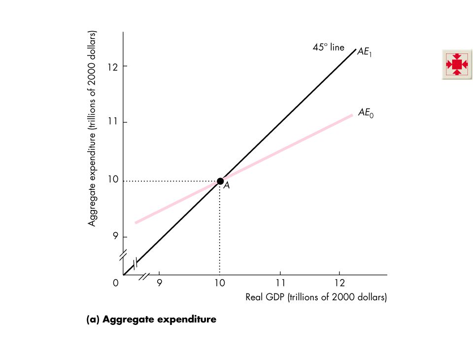
In Figure 29.10(a), a rise in price level from 105 to 125 shifts the AE curve from AE0 downward to AE1 and decreases the equilibrium level of real output from $10 trillion to $9 trillion.
The mechanics of the relationship between the AE and AD curves. Students need a lot of help and clear explanation of the mechanics of the link between these two curves. Here’s what to stress:
1. The AE curve shows how aggregate planned expenditure depends on real GDP (through the effects of disposable income), other things remaining the same.
2. The AD curve shows how equilibrium aggregate expenditure depends on the price level, other things remaining the same.
The next two points are really hard for students:
3. A change in the price level changes autonomous expenditure, which shifts the AE curve, generates a new level of equilibrium expenditure, and generates a new point on the AD curve—Figure
4. A change in autonomous expenditure at a given price level shifts the AE curve, generates a new level of equilibrium expenditure, and shifts the AD curve by an amount equal to the change in autonomous expenditure multiplied by the multiplier.
Explain these last two points very painstakingly and illustrate them with Figure and Figure

70. The Multiplier and the Price Level
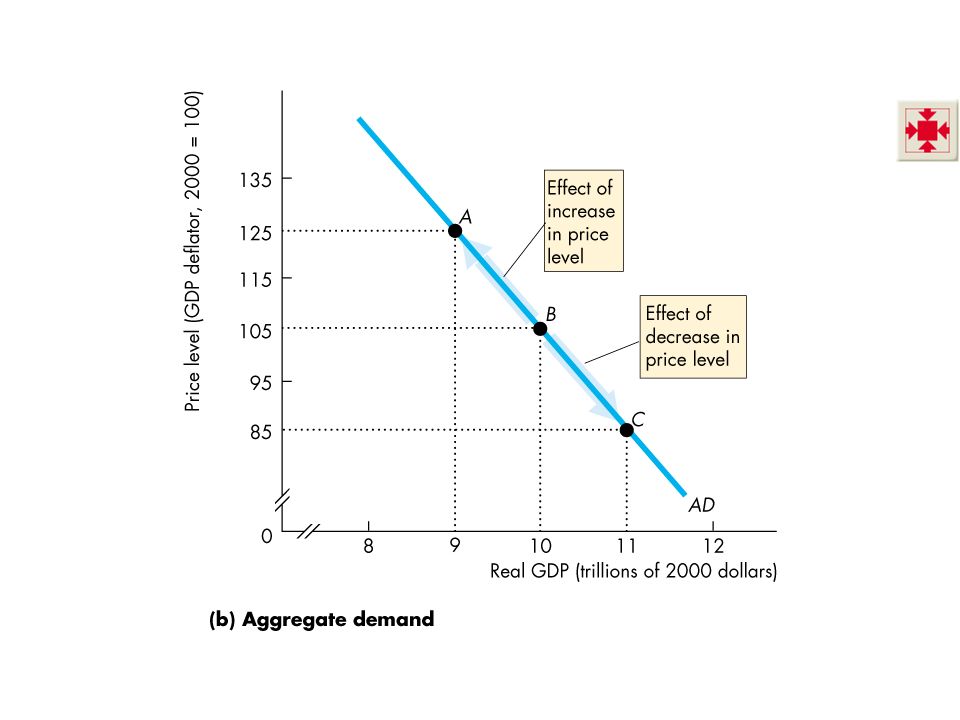
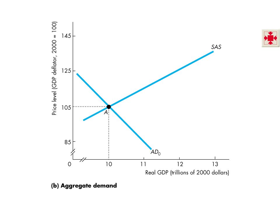
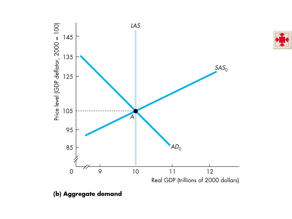
In Figure 29.10(b), the same rise in the price level that lowers equilibrium expenditure, brings a movement along the AD curve to point A.

72. The Multiplier and the Price Level
A fall in price level from 110 to 85 shifts the AE curve from AE0 upward to AE2 and increases equilibrium real GDP from $10 trillion to $11 trillion.

75. The Multiplier and the Price Level
A fall in price level from 110 to 85 shifts the AE curve from AE0 upward to AE2 and increases equilibrium real GDP from $10 trillion to $11 trillion.
The same fall in the price level that raises equilibrium expenditure brings a movement along the AD curve to point C.

78. The Multiplier and the Price Level
Points A, B, and C on the AD curve correspond to the equilibrium expenditure points A, B, and C at the intersection of the AE curve and the 45° line.

81. The Multiplier and the Price Level
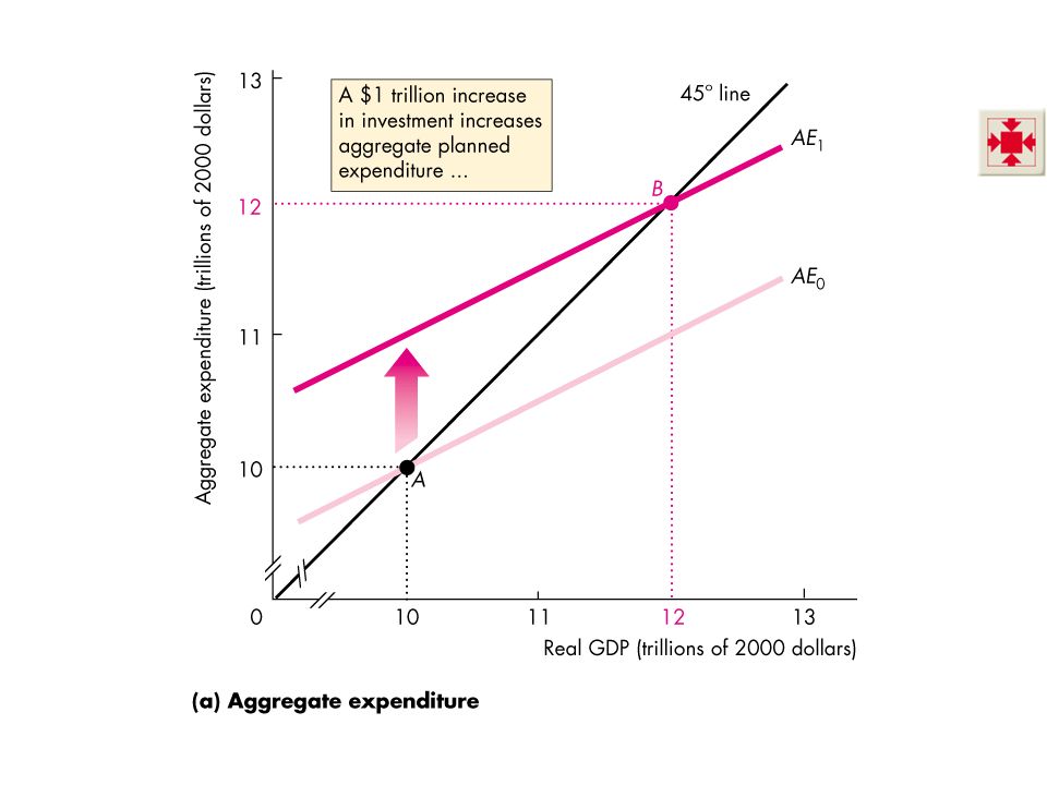
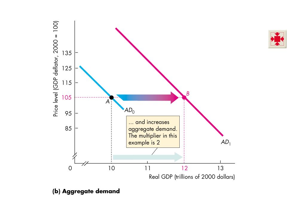
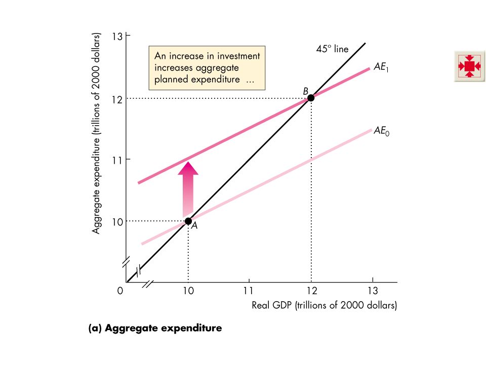
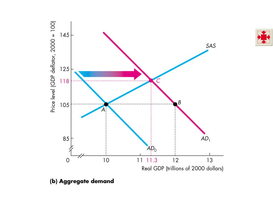
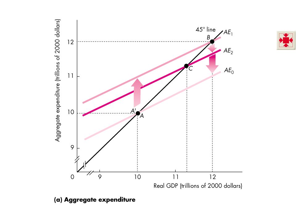
Figure illustrates the effects of an increase in autonomous expenditure.
An increase in autonomous expenditure shifts the aggregate expenditure curve upward and shifts the aggregate demand curve rightward by the multiplied increase in equilibrium expenditure.

84. The Multiplier and the Price Level
Equilibrium Real GDP and the Price Level
Figure shows the effect of an increase in investment in the short run when the prices level changes and the economy moves along its SAS curve.
The key point. Emphasize the key point of this section: That the AE model and the multiplier tell us how far the AD curve shifts when autonomous expenditure changes and the multiplier process as expenditure and GDP respond to unplanned changes in inventories bring real GDP and the price level to a new equilibrium.

87. The Multiplier and the Price Level
The increase in investment shifts the AE curve upward…
… and shifts the AD curve rightward.
With no change in the price level real GDP would increase to $12 trillion at point B.

90. The Multiplier and the Price Level
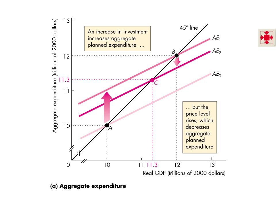
The AD curve shifts rightward by the amount of the multiplier effect but equilibrium real GDP increases by less than this amount because the price level rises.

93. The Multiplier and the Price Level
Real GDP increases from $10 trillion from $11.3 trillion, instead of to $12 trillion as it does with a fixed price level.

96. The Multiplier and the Price Level
Figure illustrates the long-run effects of an increase in autonomous expenditure at full employment.

99. The Multiplier and the Price Level
If the increase in autonomous expenditure takes real GDP above potential GDP.
The money wage rate rises, the SAS curve shifts leftward, and real GDP decreases until it is back at potential real GDP.
The long-run multiplier is zero.
The multiplier in the long run. This analysis is a repeat of what you covered earlier in the AS-AD chapter and is reinforcement. The key point to emphasize is that there is no multiplier if we start at full employment.
The multiplier is not an empirically relevant concept until it is combined with information about the state of the economy relative to full employment.

102. THE END