3. Measures of central tendency are statistics that express the most typical or average scores in a distribution These measures are: The Mode The Median The Mean The simplest measure of central tendency is the mode; the mode is the value that occurs with the greatest frequency within a data set Sample A (g) 1.42 1.431.44 1.451.46 Sample B (g) 1.361.371.401.431.44 1.471.481.492.01 Students weighed two different samples of broad beans and obtained the data shown below

4. Sample A (g) 1.42 1.431.44 1.451.46 Sample B (g) 1.361.371.401.431.44 1.471.481.492.01 Students weighed two different samples of broad beans and obtained the data shown below The most frequently occurring value (i.e. the mode) in both Sample A and Sample B is 1.44 The Median is the central or middle value of a set of values when placed in order 1.42 1.42 1.43 1.44 1.44 1.44 1.44 1.45 1.46 1.46 Sample A Median As sample A includes an even number of values then the median is halfway between the middle two, i.e. 1.44 and 1.44; these values are the same and the median is therefore 1.44

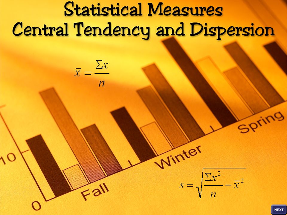
5. Sample A (g) 1.42 1.431.44 1.451.46 Sample B (g) 1.361.371.401.431.44 1.471.481.492.01 The Mean is obtained by adding up all of the values and then dividing their sum by the number of values The formula for calculating the mean is: where x = the mean  = the sum of x = any value n = number of values Calculate the means for samples A and B

6. Sample A (g) 1.42 1.431.44 1.451.46 Sample B (g) 1.361.371.401.431.44 1.471.481.492.01 For Sample A, the mean is: 1.42 + 1.42 + 1.43 + 1.44 + 1.44 + 1.44 + 1.44 + 1.45 + 1.46 + 1.46 10 1.36 + 1.37 + 1.40 + 1.43 + 1.44 + 1.44 + 1.47 + 1.48 + 1.49 + 2.01 10 For Sample B, the mean is: Sample A Mean 14.4/10 = 1.44g Sample B Mean 14.89/10 = 1.489g

7. The Mode and Grouped Data When data is grouped, it is not possible to quote the mode precisely; the ‘modal class’ is used to describe the data The modal class for this height data is 1.51 – 1.58

8. Rule of Thumb In general, the mean is used as a measure of central tendency with quantitative (interval) data, unless the distribution is markedly skewed When summarising qualitative data, the mode or median are the most appropriate measures of central tendency When the distribution of interval data is highly skewed, then the most appropriate measure of central tendency is the median

9. Measures of central tendency alone are insufficient for characterisation of the distribution of data A measure of how much the data are dispersed or ‘spread out’ is also needed Four statistics can be used to indicate dispersion: The range The variance The standard deviation The interquartile range In most cases, the mean and standard deviation are used with quantitative (interval) data with the mode or median, and the interquartile range being used for qualitative variables

10. Standard Deviation The Standard Deviation (s) of a set of values is a measure of the spread of the values from the mean A formula for calculating the standard deviation is: where s = standard deviation x - x = the deviation of a value from the mean  = the sum of n = number of values

11. A quicker method for calculating the standard deviation is to use the equation shown below – this method is less tedious and less prone to error where s = standard deviation x = any individual value x = the mean of a set of values  = the sum of n = number of values Calculate the standard deviation for the bean samples A and B Sample A (g) 1.42 1.431.44 1.451.46 Sample B (g) 1.361.371.401.431.44 1.471.481.492.01

12. The standard deviation for Sample A is 0.013 The standard deviation for Sample B is 0.179 Sample B data displays greater variation than Sample A data

13. The standard error of the mean provides an estimate of the likelihood that a sample mean is close to the true mean of a whole population The standard error is calculated using a formula that takes into account the standard deviation of the sample (s) and the sample size (n) The formula shows that the larger the sample size, the smaller the standard error of the mean

14. Increasing the sample size by a few subjects makes a large difference to the standard error when the sample size is small, but makes much less of a difference when the sample size is large A graph of standard error of the mean against sample size reveals an interesting trend The standard error of the mean can be used to define confidence limits or intervals

15. The standard deviation of this sample was found to be 0.129 The student then estimated the standard error of the mean: The student can be 68% confident that the true mean of the population falls within the range ± 0.016 of the mean of the sample, i.e. 1.64 ± 0.016 (mean ± 1 SE) What this means is that the interval between 1.623 and 1.656 (confidence limits) has a 68% probability of containing the true mean A student measured the heights of 62 individuals and found the mean height to be 1.64 metres

16. In this case, the student can be 95% confident that the true mean of the population falls within approximately two standard errors of the mean of the sample, i.e. 1.64 ± 0.032 (mean ± 2 SE) This means that the interval between 1.608 and 1.672 (confidence limits) has a 95% probability of containing the true mean More accurate calculations make use of z scores for a normal distribution to estimate confidence intervals – for 95% confidence intervals, the standard error is multiplied by 1.96; mean ± 1.96 SE Researchers more commonly use the 95% confidence interval

17. Broad Bean Samples Estimate the standard error for Sample A and Sample B You may check your answers by entering data into a suitable statistics programme Sample A (g)Sample B (g) 1.421.36 1.421.37 1.431.40 1.441.43 1.44 1.47 1.451.48 1.461.49 1.462.01

18. The two students obtained very different statistical values from their data even though the beans had been drawn from the same population – can you suggest reasons for these differences?

19. Samples A and B are sub-groups of the total population of broad beans and may not therefore be truly representative of the population as a whole Variations between the samples and the original population may arise as a consequence of: Bias in sampling – the students may have unknowingly been selective when choosing beans to weigh – Random sampling methods should be used to eliminate bias from the results Chance – the students may have, by chance, selected a particular set of beans – this is more likely to be the case when only one sample is taken and when the sample size is small – taking at least three samples (replication), choosing appropriate sample sizes and obtaining mean results from these different samples, helps to eliminate chance effects from experimental values Measurement error – errors arising from taking any form of measurement are not uncommon – when the same material is measured or weighed on a different occasion, different values are often obtained

20. Mass of Bean Seeds (g) A group of students measured the masses of individual French bean seeds and their results are shown in the table Calculate the mean, median and mode for these results Calculate the standard deviation Estimate the standard error of the mean Define the confidence limits for the mean of this set of data Check your answers with a suitable statistics programme More Data Present these results in graphical form

23. A knowledge of the shape of the distribution of values obtained in an investigation is crucially important for choosing an appropriate statistical test for analysis The normal distribution is theoretically determined by the value of the mean and the standard deviation When the value of the mean is zero and the standard deviation is one, the normal curve is said to be in ‘standard form’ A characteristic ‘bell’ shape graph is obtained

25. Relatively few values fall into the high or low categories of the distribution; 68% of its values are within one standard deviation of the mean The characteristic bell-shaped curve of a normal distribution has the following characteristics: It is symmetrical about the mean, so that equal numbers of values fall above and below the mean (mean = median = mode) 95% of its values are within two standard deviations of the mean About 99% of its values are within three standard deviations of the mean

26. Many investigations generate data which approximate to the normal distribution

27. Skewed distributions deviate from the ‘normal’ distribution curve - their distributions are asymmetrical The mean, mode and median differ in a skewed distribution; the mean and median values are less than the mode for a negatively skewed distribution, and greater than the mode for a positively skewed distribution

28. The degree of skewness can be determined by calculating the coefficient of skewness (S k ) where s = the standard deviation When the distribution of interval data is highly skewed, then the median and interquartile range should be used as measures of central tendency and dispersion

29. A useful, visual method for assessing whether a set of data can be assumed to have come from a normal distribution is to plot the data against their cumulative frequency distribution on special graph paper The graph paper used for this plot is called normal probability paper When the graphed data lies close to a straight line, we may assume that the distribution is approximately normal

30. Class Interval (m) Frequency Cumulative Frequency Percentage Cumulative Frequency 1.30 – 1.373 1.37 – 1.4412 1.44 – 1.5114 1.51 – 1.5824 1.58 – 1.6523 1.65 – 1.7222 1.72 – 1.7916 1.79 – 1.866 Use the human height data above to obtain the cumulative frequencies and the percentage cumulative frequencies Percentage cumulative frequencies are obtained by dividing the cumulative frequencies by the total cumulative frequency and multiplying by 100

31. Class Interval (m) Frequency Cumulative Frequency Percentage Cumulative Frequency 1.30 – 1.37332.50 1.37 – 1.44121512.50 1.44 – 1.51142924.17 1.51 – 1.58245344.17 1.58 – 1.65237663.33 1.65 – 1.72229881.67 1.72 – 1.791611495.00 1.79 – 1.866120100.00 Plot a graph of percentage cumulative frequency against the upper class boundary of the height data using the provided probability graph paper Assess the normality of the distribution for the height data

32. The probability plot for the height data shows that the points lie close to a straight line, and we may assume that the distribution is approximately normal Using the same method, test the bean data on the following slide for normality

33. Class Interval (g)Frequency Cumulative Frequency Percentage Cumulative Frequency 0.91 - 1.04222.86 1.04 - 1.175710.00 1.17 - 1.3051217.14 1.30 - 1.43142637.14 1.43 - 1.56133955.71 1.56 - 1.69115071.43 1.69 - 1.8295984.29 1.82 - 1.9576694.29 1.95 - 2.0816795.71 2.08 - 2.21370100.00 BEAN DATA

34. The probability plot for the bean data shows that the points lie close to a straight line, and we may assume that the distribution is approximately normal