Download presentation
Presentation is loading. Please wait.

1
Multiple Comparisons

2
Multiple Range Tests Tukey’s and Duncan’s Orthogonal Contrasts

3
Orthogonal Contrasts

4
AOV Orthogonal Contrasts

5
Tukey’s Multiple Range Test

6
Consider that cultivars A and B were developed in Idaho and C and D developed in California Do the two Idaho cultivars have the same yield potential? Do the two California cultivars have the same yield potential? Are Idaho cultivars higher yielding than California cultivars?

7
Analysis of Variance

8
Orthogonality c i = 0 [c 1i x c 2i ] = 0 c i = 0 -1 -1 +1 +1 -- c i = 0 c i = 0 -1 +1 -1 +1 -- c i = 0 c i = 0 +1 -1 -1 +1 -- c i = 0
![Orthogonality c i = 0 [c 1i x c 2i ] = 0 c i = c i = 0 c i = c i = 0 c i = c i = 0](http://images.slideplayer.com/25/8158665/slides/slide_8.jpg "Orthogonality c i = 0 [c 1i x c 2i ] = 0 c i = c i = 0 c i = c i = 0 c i = c i = 0")
9
Calculating Orthogonal Contrasts d.f. (single contrast) = 1 S.Sq(contrast) = M.Sq = [ c i x Y i ] 2 /n c i 2 ]
 = 1 S.Sq(contrast) = M.Sq = [ c i x Y i ] 2 /n c i 2 ].")
10
Orthogonal Contrasts - Example

11
S.Sq = [ c i x Y i ]/[n c i 2 ] S.Sq(1) [(-1)64.1+(-1)76.6+(1)40.1+(1)47.8] 2 / n c i 2 = 52.8 2 /(3 x 4) = 232.32
![S.Sq = [ c i x Y i ]/[n c i 2 ] S.Sq(1) [(-1)64.1+(-1)76.6+(1)40.1+(1)47.8] 2 / n c i 2 = /(3 x 4) =](http://images.slideplayer.com/25/8158665/slides/slide_11.jpg "S.Sq = [ c i x Y i ]/[n c i 2 ] S.Sq(1) [(-1)64.1+(-1)76.6+(1)40.1+(1)47.8] 2 / n c i 2 = /(3 x 4) =")
12
S.Sq(2) [(-1) x 64.1+(+1) x 76.6] 2 /(3x2) 26.04 S.Sq(3) [(-1) x 40.1+(+1) x 47.8] 2 /(3x2) 9.88
![S.Sq(2) [(-1) x 64.1+(+1) x 76.6] 2 /(3x2) S.Sq(3) [(-1) x 40.1+(+1) x 47.8] 2 /(3x2) 9.88](http://images.slideplayer.com/25/8158665/slides/slide_12.jpg "S.Sq(2) [(-1) x 64.1+(+1) x 76.6] 2 /(3x2) S.Sq(3) [(-1) x 40.1+(+1) x 47.8] 2 /(3x2) 9.88")
13
Orthogonal Contrasts

14
Five dry bean cultivars (A, B, C, D, and E). Cultivars A and B are drought susceptible. Cultivars C, D and E are drought resistant. Four Replicate RCB, one location Limited irrigation applied.

15
Analysis of Variance

16
Orthogonal Contrast Example #2 Tukey’s Multiple Range Test

17
Orthogonal Contrasts Is there any difference in yield potential between drought resistant and susceptible cultivars? Is there any difference in yield potential between the two drought susceptible cultivars? Are there any differences in yield potential between the three drought resistant cultivars?

18
Orthogonal Contrasts

19
S.Sq(1)= [(-3)130+(-3)124+(2)141+(2)186+(2)119] 2 /n c i 2 130 2 /(4 x 40) = 140.8 S.Sq(2)= [(-1)130+(+1)124] 2 /n c i 2 6 2 /(4 x 2) = 4.5 S.Sq(Rem) = S.Sq(Cult)-S.Sq(1)-S.Sq(2) 728.2-140.8-4.5 = 582.9 (with 2 d.f.)
![S.Sq(1)= [(-3)130+(-3)124+(2)141+(2)186+(2)119] 2 /n c i /(4 x 40) = S.Sq(2)= [(-1)130+(+1)124] 2 /n c i /(4 x 2) = 4.5 S.Sq(Rem) = S.Sq(Cult)-S.Sq(1)-S.Sq(2) = (with 2 d.f.)](http://images.slideplayer.com/25/8158665/slides/slide_19.jpg "S.Sq(1)= [(-3)130+(-3)124+(2)141+(2)186+(2)119] 2 /n c i /(4 x 40) = S.Sq(2)= [(-1)130+(+1)124] 2 /n c i /(4 x 2) = 4.5 S.Sq(Rem) = S.Sq(Cult)-S.Sq(1)-S.Sq(2) = (with 2 d.f.)")
20
Analysis of Variance

21
Partition Contrast(rem)
")
22
Analysis of Variance

23
Alternative Contrasts

24
S.Sq(1)= [(-3)130+(-3)124+(2)141+(2)186+(2)119] 2 /n c i 2 130 2 /(4 x 40) = 140.8 S.Sq(2)= [(-1)130+(-1)124+(-1)141+(4)186+(-1)119] 2 /n c i 2 230 2 /(4 x 20) = 661.2 S.Sq(Rem) = S.Sq(Cult)-S.Sq(1)-S.Sq(2) 728.2-140.8-661.2 = -73.8 (Oops !!!) (with 2 d.f.)
![S.Sq(1)= [(-3)130+(-3)124+(2)141+(2)186+(2)119] 2 /n c i /(4 x 40) = S.Sq(2)= [(-1)130+(-1)124+(-1)141+(4)186+(-1)119] 2 /n c i /(4 x 20) = S.Sq(Rem) = S.Sq(Cult)-S.Sq(1)-S.Sq(2) = (Oops !!!) (with 2 d.f.)](http://images.slideplayer.com/25/8158665/slides/slide_24.jpg "S.Sq(1)= [(-3)130+(-3)124+(2)141+(2)186+(2)119] 2 /n c i /(4 x 40) = S.Sq(2)= [(-1)130+(-1)124+(-1)141+(4)186+(-1)119] 2 /n c i /(4 x 20) = S.Sq(Rem) = S.Sq(Cult)-S.Sq(1)-S.Sq(2) = (Oops !!!) (with 2 d.f.)")
25
c 1i = 0 (-3) + (-3) + (+2) + (+2) + (+2) = 0 = c 2i = 0 (-1) + (-1) + (-1) + (+4) + (-1) = 0 = [c 1i x c 2i ] = 0 (-3)(-1)+(-3)(-1)+2(-1)+2(4)+2(-1) =10 = Orthogonality
![ c 1i = 0 (-3) + (-3) + (+2) + (+2) + (+2) = 0 = c 2i = 0 (-1) + (-1) + (-1) + (+4) + (-1) = 0 = [c 1i x c 2i ] = 0 (-3)(-1)+(-3)(-1)+2(-1)+2(4)+2(-1) =10 = Orthogonality](http://images.slideplayer.com/25/8158665/slides/slide_25.jpg " c 1i = 0 (-3) + (-3) + (+2) + (+2) + (+2) = 0 = c 2i = 0 (-1) + (-1) + (-1) + (+4) + (-1) = 0 = [c 1i x c 2i ] = 0 (-3)(-1)+(-3)(-1)+2(-1)+2(4)+2(-1) =10 = Orthogonality")
26
More Appropriate Contrasts

27
Analysis of Variance

28
Conclusions Almost all the variation between cultivars is accounted for by the difference between cv ‘D’ and the others. The remaining 4 cultivars are not significantly different. Orthogonal contrast result is exactly the same are the result from Tukey’s contrasts.

29
Conclusions Important to make the “correct” orthogonal contrasts. Important to make contrasts which have “biological sense”. Orthogonal contrasts should be decided prior to analyses and not dependant on the data.

30
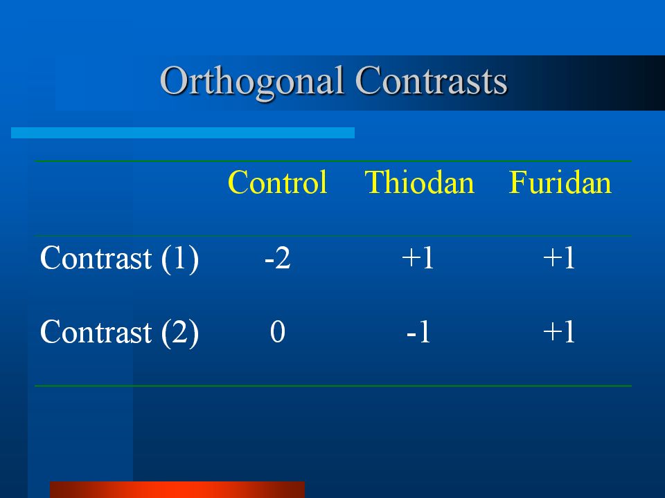
Orthogonal Contrasts Four Brassica species (B. napus, B. rapa, B. juncea, and S. alba). Ten cultivars ‘nested’ within each species. Three insecticide treatments (Thiodan, Furidan, no insecticide). Three replicate split-plot design.
. Ten cultivars ‘nested’ within each species. Three insecticide treatments (Thiodan, Furidan, no insecticide). Three replicate split-plot design..")
31
Analysis of Variance

32
Species and Treatment Means

33
Orthogonal Contrasts

35
Analysis of Variance

36
Species x Treatment Interaction

37
Species x Contrast (1)
")
38
Species x Contrast (2)
")
39
Orthogonal Contrasts and Interactions Consider a cross classified factorial design with 4 replicates. Four cultivars; 2 from Idaho and 2 from California (again). 3 herbicide treatments; No-treatment control, Killall, and Onllik.
. 3 herbicide treatments; No-treatment control, Killall, and Onllik..")
40
Cultivar ControlKillallOnllikTotal IdaBest 90168147405 IdaCream 75141135351 Yuppy 456475184 Total 210373357 Orthogonal Contrasts and Interactions

41
Contrasts for cultivars? Idaho v California (-1 -1 +2), SS(Id v CA) = 2,787; Contrast for herbicides? Herbicide v No-treatment control (-2 +1 +1), SS(Herb v Not) = 1,779; Contrast for the interaction between the first two contrasts?
, SS(Id v CA) = 2,787; Contrast for herbicides. Herbicide v No-treatment control ( ), SS(Herb v Not) = 1,779; Contrast for the interaction between the first two contrasts .")
42
GenotypeHerb YieldID v CA Herb v Not Interaction IdaBestCont 90 IdaBestKillall 168 IdaBestOnllik 147 IdaCreamCont 75 IdaCreamKillall 141 IdaCreamOnllik 135 YuppyCont 45 YuppyKillall 64 YuppyOnllik 75 Orthogonal Contrasts and Interactions

43
GenotypeHerb YieldID v CA Herb v Not Interaction IdaBestCont 90 IdaBestKillall 168 IdaBestOnllik 147 IdaCreamCont 75 IdaCreamKillall 141 IdaCreamOnllik 135 YuppyCont 45+2 YuppyKillall 64+2 YuppyOnllik 75+2 Orthogonal Contrasts and Interactions

44
GenotypeHerb YieldID v CA Herb v Not Interaction IdaBestCont 90-2 IdaBestKillall 168+1 IdaBestOnllik 147+1 IdaCreamCont 75-2 IdaCreamKillall 141+1 IdaCreamOnllik 135+1 YuppyCont 45+2-2 YuppyKillall 64+2+1 YuppyOnllik 75+2+1 Orthogonal Contrasts and Interactions

45
GenotypeHerb YieldID v CA Herb v Not Interaction IdaBestCont 90-2+2 IdaBestKillall 168+1 IdaBestOnllik 147+1 IdaCreamCont 75-2+2 IdaCreamKillall 141+1 IdaCreamOnllik 135+1 YuppyCont 45+2-2-4 YuppyKillall 64+2+1+2 YuppyOnllik 75+2+1+2 Orthogonal Contrasts and Interactions

46
Contrasts for cultivars? Idaho v California (-1 -1 +2), SS(Id v CA) = 2,787; Contrast for herbicides? Herbicide v No-treatment control (-2 +1 +1), SS(Herb v Not) = 1,779; Contrast for the interaction between the first two contrasts? SS (Interaction) = 246.
, SS(Id v CA) = 2,787; Contrast for herbicides. Herbicide v No-treatment control ( ), SS(Herb v Not) = 1,779; Contrast for the interaction between the first two contrasts. SS (Interaction) =")
47
Orthogonal Contrasts and Interactions

48
More Orthogonal Contrasts … Trend Analyses

49
Aim of Analyses of Variance Detect significant differences between treatment means. Determine trends that may exist as a result of varying specific factor levels.

50
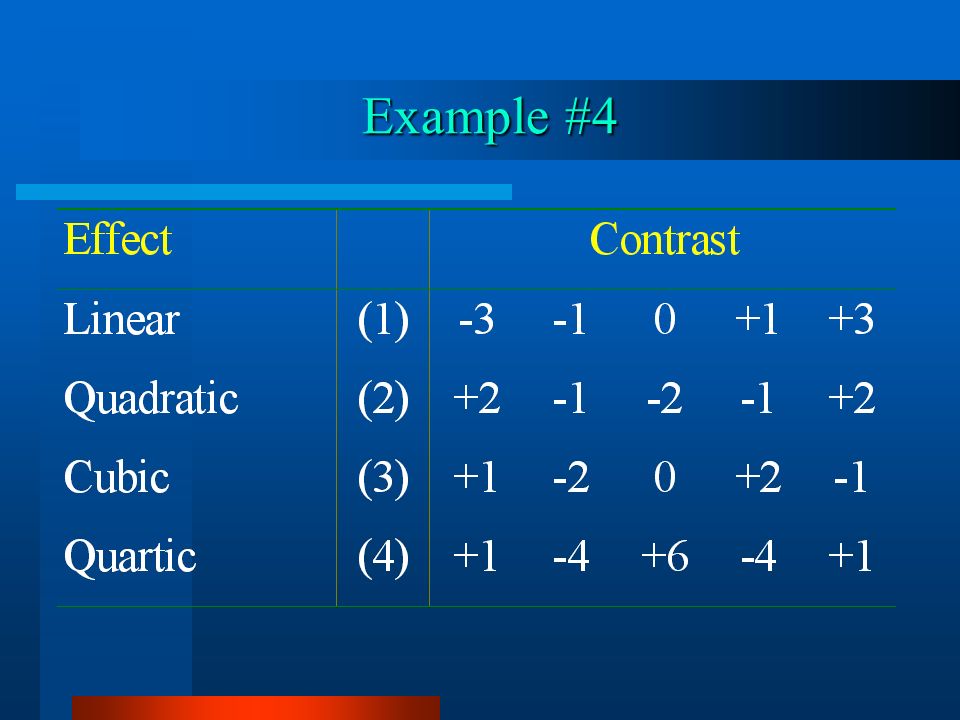
Example #4 Ten yellow mustard (S. alba) cultivars. Five different nitrogen application rates (50, 75, 100, 125, and 150)
.")
51
Analysis of Variance

52
Orthogonal Contrasts

53
Example #4

56
Analysis of Variance

57
Trend Analyses The F-value associates with a trend contrast is significant. All higher order trend contrasts are not significant.

58
Example #4

59
Linear

60
Quadratic

61
Cubic

62
Quartic

63
Example #5 Two carrot cultivars (‘Orange Gold’ and ‘Bugs Delight’. Four seeding rates (1.5, 2.0, 2.5 and 3.0 lb/acre). Three replicates.
. Three replicates..")
64
Example #5

65
Analysis of Variance

67
Orange Gold Bug’s Delight

68
End of Analyses of Variance Section

Similar presentations


>")
 Environmental sampling and analysis.>")


 factorial with n = 5 replicate Total number of observations:>")


. Two Factor Analysis of Variance Main effect The effect of a single factor when any other factor is ignored. Example.>")