1. Course outline, objectives, workload, projects, expectations Introductions Remote Sensing Overview Elements of a remote sensing observing system 1. platform (satellite, surface, etc) 2. experimental design - forward problem 3.retrieval components - inversion/estimation http://reef.atmos.colostate.edu/~odell/at652/

2. Why remote sensing? Much of the atmosphere is inaccessible to routine in situ measurements  Only way to provide large enough sample to provide a large-scale view of the Earth system is from space AVHRR SST anomalies Nov 96,97

4. Related Classes AT721 – Advanced Techniques in Radiative Transfer Spring 2014, O’Dell Will focus on RT techniques in various parts of the spectrum, with application primarily to remote sensing but also energy budget. Bulk of the class is a single large application-based project of the student’s choice. AT752 – Inverse methods in the atmoospheric sciences (Fall 2014, O’Dell) Fall 2014, O’Dell Provides an introduction to inverse modeling, with application to modern retrieval theory, flux inversions, and data assimilation. AT737 – Satellite Observations Spring 2015?, VonderHaar Satellite measurements; basic orbits and observing systems; applications of remote sensing and imaging to investigations of atmospheric processes.

5. UCAR Comet Lectures We will occasionally draw on lecture material from the UCAR Comet “MetEd” series, either in place of class or out of class.

6. What is remote sensing? “The observation of radiation* that interacted with a remote object or collection of objects” Does not mean satellites specifically! (surface, ballon- borne, etc can also count) Usually it is the amount of radiation that matters, but sometimes timing is also used (e.g. radar & lidar) * Some don’t use radiation (e.g. GRACE uses gravity field)

7. Properties of the earth system that are subject to remote sensing Temperature: land surface, ocean surface, atmospheric profile (troposphere & stratosphere) Gases: water vapor, ozone, CO 2, methane, oxygen, NO 2, CO, BrO, D 2 O,... (integrated & profile info) Clouds: Optical depth, cloud profile, particle sizes, ice vs. liquid (phase), cloud fraction Aerosols: Types (sulfates, sea salt, dust, smoke, organics, black carbon), optical depth, height Surface features: surface height, ocean winds, vegetation properties, ocean color, sea ice, snow cover.

8. Applications?

9. Weather prediction (data assimilation) Climate state observations (e.g. clouds, sea ice loss) Climate Model validation/comparisons Air quality state / forecasts Solar power forecasts Carbon cycle Hydrology/water cycle Biogeochemical modeling

10. Example: Data assimilation for NWP ECMWF assimilated data breakdown

11. 11 “Golden Age of Remote Sensing” NASA’s A-Train

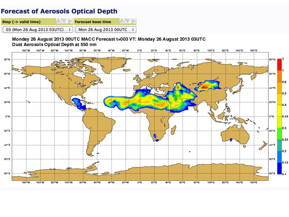
12. Example: Monitoring of Atmospheric Composition & Climate (MACC) at ECMWF

14. Carbon Monoxide Forecast

16. “Cloud Streets” over near Greenland from MODIS

17. Monitoring Climate Change: Stratospheric cooling & tropospheric warming with microwave O 2 17

18. A puzzle?

19. There are multiple aspects to remote sensing: Platform (aircraft, satellite, balloon, ground- based) – this dictates the time/space sampling characteristics & errors Source of EM Radiation Radiation interaction mechanism Forward and inverse models - this defines the physical and system errors (user in principle has more control over this facet of the system)

20. Observing Platforms Ground-based: Radiometers, sunphotometers, lidar, radar, doppler wind arrays. Local but good time coverage. Aircraft: local-to-regional spatial, limited time coverage (measurement campaigns) Satellite (orbit determines spatial & temporal coverage)

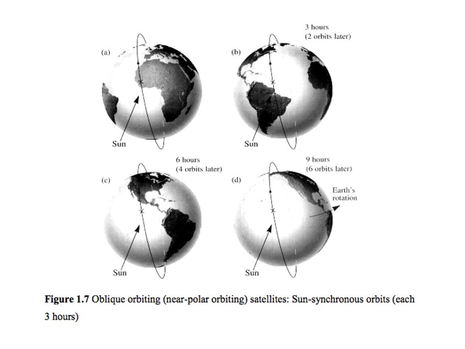
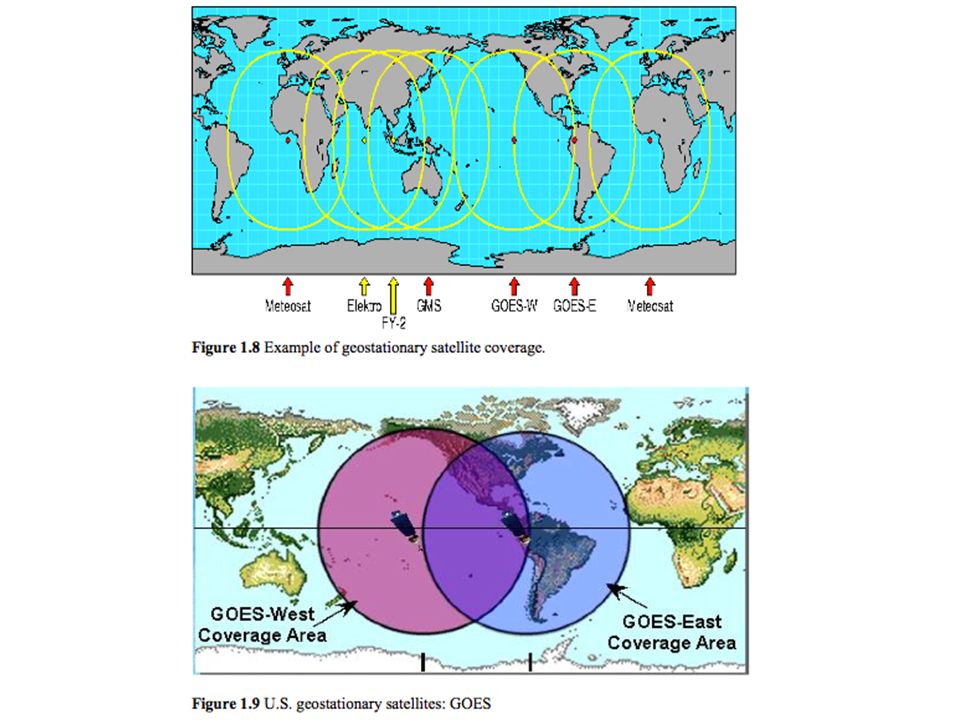
21. Substantial influence on sampling - e.g. synoptic like versus asynoptic

24. HEO Example: PCW-PHEMOS from Environment Canada Trischenko & Garand (2011) Polar Communications and Weather (PCW) mission (2017): 2 operational met satellites in Highly Elliptical Orbit (HEO) for quasi-geostationary observations along with a communications package Polar Highly Elliptical Molniya Orbit Science (PHEMOS) suite of imaging spectrometers Weather Climate and Air quality (WCA) option is now entering phase-A study (see talk by J.C. McConnell on Thursday) Quasi-continuous coverage of GHGs over the high latitudes (~40-90°N) using TIR+NIR would help constrain GHG sources/sinks at fine temporal scales Courtesy Ray Nassar

25. Source of Radiation PASSIVE Sunlight (UV, Vis, Near IR): May be scattered (by atmospheric constituents or surface) or absorbed. Thermal Emission (Thermal IR, microwave, radio) ACTIVE Radar (radio & microwave), GPS (radio) Lidar (visible and near-infrared)

26. Radiation Interactions Extinction Radiation removed from some background source (typically the sun or a laser) Can be removed because of scattering, absorption, or both Emission Adds radiation to a beam because of THERMAL EMISSION (thermal IR & microwave only) Scattering Adds radiation to a beam From clouds, aerosols, or surface. Affects solar & thermal Passive or active

27. Experimental Design Based on some sort of relation defined by a physical process: (a) extinction – aerosol OD, TCCON CO2, occultation (b) emission - atmospheric sounding, precipitation,.. (c) scattering - passive, cloud aerosol, ozone,.. - active, radar & lidar

28. The Observing System Transfer Function Key parameters & steps : Measurement, y(t) and error  y Model f & its error  f Model parameters b and errors Constraint parameters c Physical Variables (T, q, etc) Radiation Signal Inferred Physical Variables + UNCERTAINTI ES!

29. The Retrieval Problem Forward Problem (real) y=F(x) +  y y = measurement F = Nature’s forward model x = parameter desired ε y = error in measurement (noise, calibration error,…) b = ‘model’ parameters that facilitate evaluation of f  f = error of model Often the relation between the measurement y and the parameter of interest x is not entirely understood y=f(,b) +  y +  f Inverse Problem

30. PROBLEM: The performance of the ‘system’ is affected by the performance of the individual parts. Examples of issues: (i)Properly formed forward models – [e.g. Z-R relationships, poorly formed forward model without an understanding of what establishes the links between the observable y(Z) and the retrieved parameter X(R) ] (ii) Need for prior constraints – temperature inversion problem (iii) Poorly formed inverse model: simple regressions or neural network systems might not produce useful errors

31. Inversion versus estimation - radar/rainfall example Radar -rainfall relationship Z= AR b ‘Inversion’ R= (Z/A) 1/b but…… A and b are not-unique and vary from rain-type to rain-type implicitly involving some sort of ‘cloud’ model Stephens, 1994

32. Non-uniqueness and Instability Estimation Cost Function:  = M [y-f(x)] measurement Prediction of measurement ‘metric’ of length (e.g. least squares) Unconstrained Constrained x2x2 x1x1 Solution space non-unique x2x2 x1x1  = M [y-f(x)] + C(x) M M C C(x)= initial or a priori constraint

33. Physically: Weighting functions that substantially overlap I(0) =  B(z’)W(0,z’)dz’ 1 2 z Non-uniqueness and instability: example from emission Will generally not yield unique solution in the presence of instrument noise & finite # of channels

34. Results from temperature retrieval project Noiseless Retrieval Realistic noise, assumed noiseless Realistic noise, proper noise model Weighting Functions from a theoretical instrument

35. Information Content: The example of IR-based retrieval of water vapor Metric of how much a priori constraint contribute to the retrieval A  0, all a priori, no measurement A  1, no a priori, all measurement

36. Change Calibration (i.e. measurement error by 100%) error Largest impact where measurements contribute most

37. Forward Problem (applied) y = f( ) +  y +  f f = our depiction of the forward model = estimates of x,y  f = F(x,b) - f ( ) +, = error in forward model Radiative transfer model (most common) Radiation + physical model Radiation model + NWP (radiance assimilation) For the most challenging problems we encounter, it is generally true that the largest uncertainty arise from forward model errors. If you see error estimates on products that exclude these errors – then you ought to be suspicious – really suspicious

38. Geostationary allows us to see cloud mov