1. Altred Wegener Institut, Bremerhaven, 4. Juli 2005 Klimasimulationen der letzten 1000 Jahre - was man daraus lernen kann Institute für Küstenforschung GKSS, Geesthacht Hans von Storch and Eduardo Zorita

2. Abstract A series of multicentury simulations with the global climate model ECHO-G have been performed to generate a realistic mix of natural and externally (greenhouse gases, solar output, volcanic load) forced climate variations. Among others, these simulations are used to examine the performance of empirically based methods to reconstruct historical climate. This is done by deriving from the model output “pseudo proxies”, which provide incomplete and spatially limited evidence about the global distribution of a variable. These pseudo proxies serve as input in reconstruction methods – the result of which can then be compared with the true state simulated by the model. The questions we have dealt with are: a)Is the MBH method (commonly known as hockeystick method) reliable in reconstructing low-frequency variability? b)Is the phenomenon, that an EOF analysis of a field of spatially incoherent, time wise red noise variables sometimes returns artificial hockey sticks when the time centering is done for a sub-period, relevant when applied to historical situations? c)Is the skill of the reconstruction on multi-decadal and centennial time scales significantly increased if the spatial density of proxy data is increased? d)Can a reconstruction be improved when longer time series are available?

3. Motivation: the failed quest for low- dimensional nonlinearity in 1986 In the 19070s and 80s, scientists were eager to identify multi-modality of atmospheric dynamics – as a proof that low-dimensional system’s theory is applicable to atmospheric dynamics. Hansen, A.R. and A. Sutera, 1986: On the probability density function of planetary scale atmospheric wave amplitude. J. Atmos. Sci. 43 – made widely accepted claims for having detected bimodality in data representative for planetary scale dynamics. J.M. Wallace initiated a careful review – and found the claim exaggerated because of methodical insufficiencies: Nitsche, G., J.M. Wallace and C. Kooperberg, 1994, J. Atmos. Sci. 51. Alleged proof for bi-modality of extratropical atmospheric dynamics

4. Motivation: the failed quest for low- dimensional nonlinearity in 1986 ● - From the case of 1986 the scientific community has learned that it is wise to be reluctant before accepting wide-reaching claims which are based on purportedly advanced and complex statistical methods. ● - Statistical analysis does not provide magic bullets. After a real pattern has been detected with an allegedly advanced method, it must be identifiable also with simpler methods.

5. We have used a millennial simulation to examine the questions … Is the hockey stick method reliable in reconstructing low-frequency variability? Is the phenomenon that an EOF analysis of a field of spatially incoherent, time wise red noise variables sometimes returns artificial hockey sticks when the time centering is done for a sub-period, relevant when applied to historical situations? Is the skill of the reconstruction on multi- decadal and centennial time scales significantly increased if the spatial density of proxy data is increased? Can a reconstruction be improved when longer time series are available?

6. Quasi-realistic Climate Models … Climate = statistics of weather. Quasi-realistic climate models (as opposed to reduced climate models, e.g., EBM’s) feature dynamics of troposphere, ocean, sea ice + more. Grid size typically  200 km and time step  0.5 hrs. Such models are considered to realistically describe - climate variability of time scales between hours and centuries, and > 800 km (or so) - the climate conditional upon (some?) external factors

7. ECHO-G simulations „Erik den Røde” (1000- 1990) and “Christoph Columbus” (1550-1990) with estimated volcanic, GHG and solar forcing

8. 1675-1710 vs. 1550-1800 Reconstruction from historical evidence, from Luterbacher et al. Late Maunder Minimum Model-based reconstuction

9. A more systematic comparison of the ECHO-G performance with various proxy data – during the Late Maunder Minimum episode (1675-1710): KIHZ-Consortium: J. Zinke, et al., 2004: Evidence for the climate during the Late Maunder Minimum from proxy data available within KIHZ. In H. Fischer et al. (Eds.): The Climate in Historical Times. Towards a synthesis of Holocene proxy data and climate models, Springer Verlag

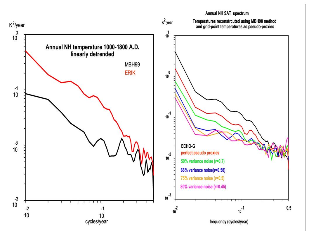
10. The millennial run generates temperature variations considerably larger than MBH-type reconstructions. The simulated temperature variations are of a similar range as derived from NH summer dendro-data, from terrestrial boreholes and low- frequency proxy data.

12. Conclusion ● “Erik den Røde”, an effort to simulate the response to estimated volcanic, GHG and solar forcing, 1000-1990. ● Low-frequency variability in Erik den Røde > Mann, Jones, and others, but ~ Esper, boreholes, Moberg, (some) instrumental data

13. Erik HadCM3 Data provided by Simon Tett. differences relative to the 1550-1800 average; 25-year running averages. Testing with HadCM3 simulation

14. Conclusion Not a specific result of ECHO-G Forcing is not particularly strong Sensitivity of ECHO- G about 2.5K Different reconstructions of solar irradiance

15. For the purpose of testing reconstruction methods, it does not really matter how „good“ the historical climate is reproduced by a millennial simulation. Such model data provide a laboratory to test MBH, McMc and other questions.

16. Testing Claims - #1 The historical development of air temperature during the past 1000 years resembles a hockey stick – with a weak ongoing decline until about 1850 and a marked increase thereafter.

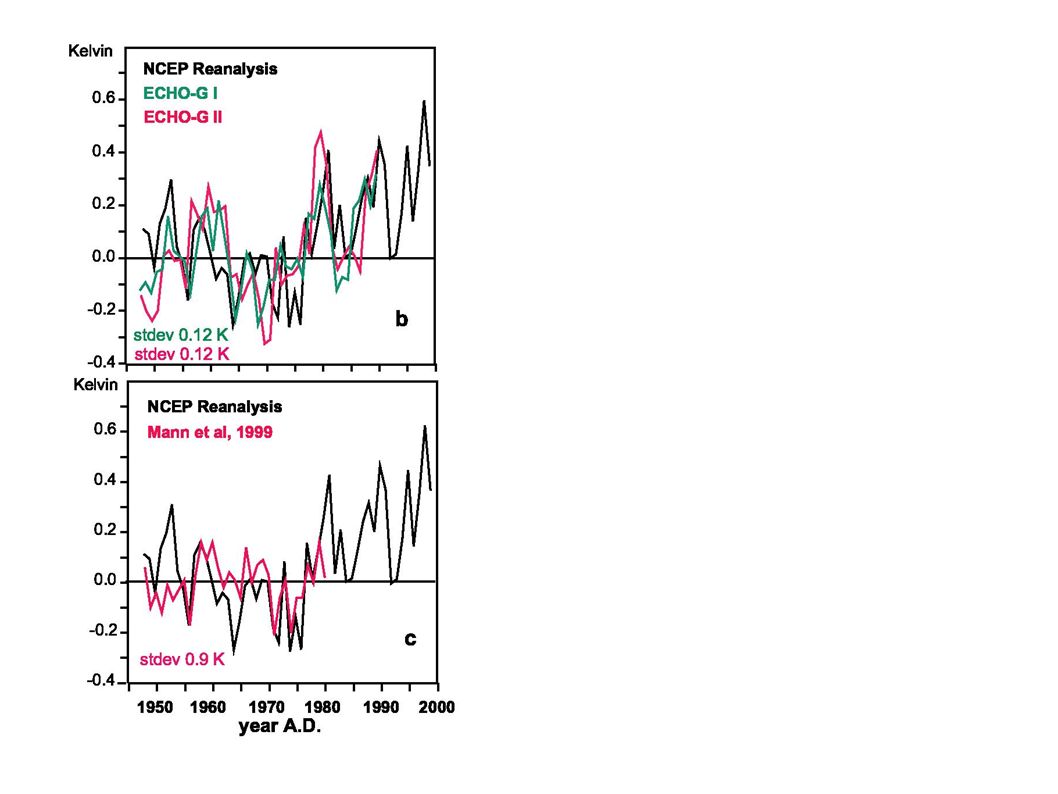
17. pseudo-proxies: grid point SAT plus white noise red: mimicking largest sample used in MBH Testing the MBH method

18. Proxy Annual values Standardization Data reduction in areas with dense network (tree-rings) through PCA Retention of leading PCs Calculation of instrumental temperature PCs Gridded T data sets Monthly anomalies Local standardization Annual mean Latitude weighting Singular value decomposition → PC i (t) and EOF i (r) Rescaling of EOF i (r) by the detrended local T standard deviation The MBH98 algorithm R Training 1902-1980 No-detrending prior to training Minimize time variance of e in: proxy_j(t) = A pc_i(t)+  (t), obtaining matrix matrix A Validation 1856-1980 Minimize spatial variance of  in: proxy j (t) = A pc i (t)+  (t) obtaining pc_i(t) for each t and number of retained PCs (depends on number of proxys available) Reconstruct temperature field by T(r)=  pc_i(t) eof_i(r) Compare with observations Reconstruction 1000-1980 Same as (4) Number of pc_i depends on period and number of proxies) ● Calculation of North Hemisphere mean from T field 1 5 4 3 2

20. Mimicking MBH?

22. Discussion Claim: MBH was not built for such large variations as in ECHO-G But – the same phenomenon emerges in a control run.

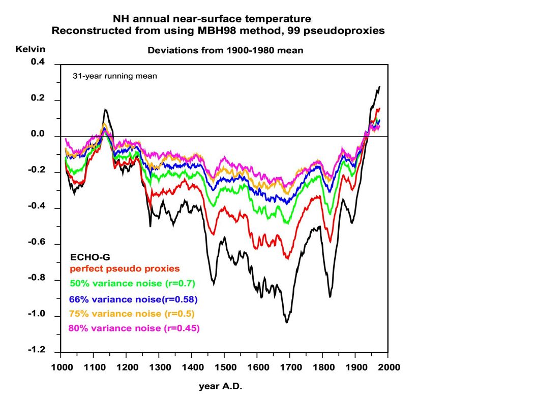
23. Training with or without trend In our implementation of MBH, the trend in the calibration period is taken out. When the trend during the calibration period is used as a critical factor in the empirical reconstruction model, then the contamination of the proxy trend by non-climatic signals must be mimicked. Thus, apart of white/red noise also error on the centennial time scale. Here: 50% centennial, 75% white noise. Again heavy underestimation of long-term variability.

24. Discussion Training MBH with or without trend in calibration period. Statistical meaningful is the exclusion of the trend, but MBH seems to exploit the trend.

25. Trend – does it really help ? If R is the reconstruction method, and S the sampling operator, then we want R·S = 1 We used the original MBH result M, given by the first 4 EOFs, and derive the MBH operator R from samples of this 1820-1890 history, including the trend. Then we compare R(S(M)) with M. The difference is significant. In case of MBH R·S ≠ 1

26. Conclusion MBH algorithm does not satisfy the basic requirement R·S = 1 Instead MBH underestimates long-term variability But R(S(E)) ≈ M, with M representing MBH and E the millennial simulation “Erik de Røde”.

27. Testing Claims - #2 McIntyre, M., and R. McKitrick, 2005: Hockey sticks, principal components and spurious significance. Geoph Res. Letters 32 Claim: Partial centering generates PC coefficients with a hockey stick pattern from red-noise random time series fields. Claim is valid – but does it matter when deriving historical reconstructions? Not included in our original analysis as we have well separated grid boxes and not clusters of proxy data (effect is potentially misleading only with respect to proxy data)

28. Conclusion Resulting from the application of the MBH98 algorithm to a network of pseudo-proxies. The variance of the pseudoproxies contains 50% noise (top panel: white noise; bottom panel: red noise with one-year lag- autocorrelation of 0.8). The pseudoproxies were subjected to separate PCA in North America, South America and Australia with full (1000-1980; red) or partial (1902-1980; blue) centering. This specific critique of McIntyre and McKitrick is irrelevant for the problem of reconstructing historical climate. (Other aspects may be, or may be not, valid.)

29. Testing Claims - #3 Hypothesis: adding more sampling locations to the procedure adds significant skill to the reconstruction. Method – training the MBH method with the largest sample available to MBH (in red) plus a number of additional sites (in blue) in Africa and Asia.

30. Conclusion The skill of the reconstruction is only marginally improved by adding additional sites.

31. Testing Claims - #4 Hypothesis – having more temporal evidence to train the reconstruction model improves the skill. Method – training the model not with 1900- 1980 but with 1680- 1720 (coldest period in the simulation) and 1900-40

32. Conclusion Some improvement, in particular when the proxies contain little noise.

33. Overall Conclusions 1.Millennial simulations are useful laboratories to test empirical methods, which can not be really validated with reliably recorded data. 2.The MBH method is associated with a systematic underestimation of long-term variability. 3.The fundamental test of reproducing the known temperature history in any millennial simulation is failed by MBH for long-term variations. 4.The McMc-phenomenon of “artificial hockey sticks” (AHS) due to unwise centering of EOFs does not cause harm for the overall process. 5.For improving historical reconstructions it is more rewarding to have additional reliable earlier data than having additional coverage in space.

34. Statistik ist nützlich